| Looks | Type I error |
|---|---|
| 1 | 0.025 |
| 2 | 0.042 |
| 3 | 0.054 |
| 5 | 0.071 |
| 10 | 0.097 |
| 20 | 0.124 |
Bayesian sequential monitoring
Posterior and predictive probabilities at each look, sequential Bayes factors, and why their frequentist error rates still have to be checked.
Posterior statements at each look
A Bayesian analysis combines a prior for the effect \(\theta\) with the data. With the normal approximation used throughout this tutorial — an estimate \(\hat\theta_k\) with information \(I_k\) — and a normal prior \(\theta \sim N(\mu_0, 1/I_0)\), the posterior at look \(k\) is
\[ \theta \mid \text{data} \sim N\!\left(\frac{I_0\mu_0 + I_k\hat\theta_k}{I_0 + I_k},\; \frac{1}{I_0 + I_k}\right). \]
The prior can be expressed as “worth \(I_0\) units of information”.
- A sceptical prior centred on no effect tempers early enthusiasm.
- An enthusiastic prior centred on \(\theta_1\) tempers early pessimism.
Reporting the conclusions under both is informative (Spiegelhalter et al. 1994).
Typical monitoring rules are:
- Efficacy: stop if \(P(\theta > \delta \mid \text{data}) \ge \gamma_E\), for a clinically relevant \(\delta\) (often 0).
- Futility: stop if the predictive probability of a successful final analysis is below \(\gamma_F\). The predictive probability averages over the data still to come, given the current posterior.
Berry (2006) reviews Bayesian clinical trials; the same ideas underlie the phase II designs of Thall and Simon (1994) and Lee and Liu (2008).
The likelihood principle does not remove the frequentist error
The posterior does not depend on the stopping rule, so a Bayesian analysis needs no multiplicity adjustment in its own terms. But the frequentist probability that a Bayesian rule declares efficacy when the treatment does not work still grows with the number of looks. With a flat prior, “stop if \(P(\theta > 0 \mid \text{data}) \ge 0.975\)” is the same as “stop if \(Z_k \ge 1.96\)”. Its type I error is that of repeated significance testing:
Regulators and journals therefore expect Bayesian sequential designs to be calibrated: their thresholds are tuned, usually by simulation, until the frequentist type I error and power are acceptable (U.S. Food and Drug Administration 2019; Stallard et al. 2020; Ryan et al. 2020).
Sequential Bayes factors
In experimental psychology, a popular alternative is the sequential Bayes factor (SBF) design. Data are added until the Bayes factor \(\mathrm{BF}_{10}\) exceeds an evidence threshold \(k\) (for \(H_1\)) or falls below \(1/k\) (for \(H_0\)) (Schönbrodt et al. 2017). For \(t\)-tests the usual choice is the default JZS prior, a Cauchy distribution on the standardised effect size (Rouder et al. 2009).
Planning uses Bayes factor design analysis: simulation of the distribution of the stopping sample size and of the rates of misleading evidence (Schönbrodt and Wagenmakers 2018). Rouder (2014) discusses how to interpret optional stopping from a Bayesian viewpoint. Stefan et al. (2022) compare the efficiency of SBF designs with the SPRT.
Example: calibrating a Bayesian design
A two-arm trial with a continuous outcome (SD 1) plans 180 patients and analyses after 60, 120 and 180. The treatment effect of interest is 0.5. The trial stops for efficacy when \(P(\theta > 0 \mid \text{data}) \ge 0.975\), and for futility when the predictive probability of that success at the end falls below 10 %. The Bayesian Sequential Monitoring analysis turns each rule into a threshold on the estimate at each look. The frequentist operating characteristics then follow exactly from the same computation as for group sequential designs:
| Prior | P(success), no effect | P(success), effect 0.5 | Expected N, no effect | Expected N, effect 0.5 |
|---|---|---|---|---|
| flat | 0.051 | 0.911 | 94.514 | 97.595 |
| sceptical | 0.021 | 0.840 | 82.824 | 112.525 |
| enthusiastic | 0.188 | 0.982 | 117.006 | 76.324 |
With a flat prior the rule is a repeated significance test at \(z = 1.96\), so its type I error is above 0.025 (futility stops pull it back a little). The sceptical prior (centred on no effect, with a 5 % chance of an effect above 0.5) demands more evidence early and keeps the type I error below 0.025; the power falls from 0.91 to 0.84. The enthusiastic prior inflates the type I error to 0.19, which is why regulators ask for these numbers.
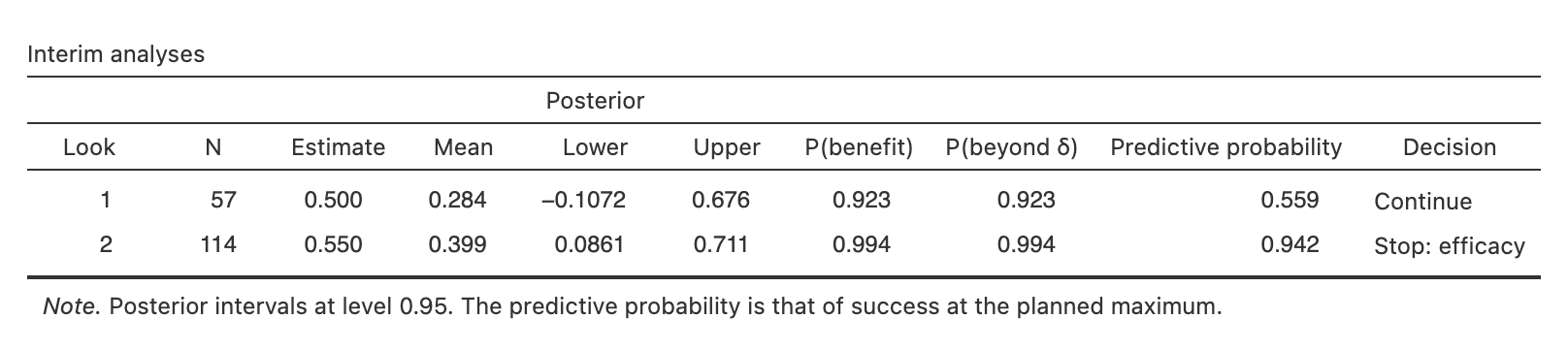
Monitoring. With the interim results of the dataset Interim analyses — difference in means and the sceptical prior, the posterior probability of benefit is 0.923 after 57 patients (continue). After 114 patients it is 0.994, above 0.975, and the trial stops for efficacy. The posterior mean, 0.40, is shrunk towards 0 from the observed 0.55.
Two arms with a binary outcome. For response rates the analysis uses Beta priors in each arm. The posterior probability \(P(p_T - p_C > \delta)\) is computed by quadrature and the predictive probability by beta-binomial sums. The operating characteristics are again exact, by following the joint distribution of the responses in both arms. The same nominal 0.975 rule with three looks (20, 40 and 60 per arm, control rate 0.3) needs a stricter threshold to keep a one-sided type I error of 0.025; among the values below, only 0.99 does:
| Success threshold | Type I error | Power |
|---|---|---|
| 0.9750 | 0.0484 | 0.6345 |
| 0.9800 | 0.0379 | 0.5876 |
| 0.9850 | 0.0297 | 0.5671 |
| 0.9900 | 0.0192 | 0.4720 |
Example: a sequential Bayes factor design
A two-sample sequential Bayes factor design tests after every patient from 10 per group, stops when \(\mathrm{BF}_{10} \ge 10\) or \(\le 1/10\), and caps the study at 100 per group (default JZS prior, \(r = 0.707\)). Bayes factor design analysis by simulation (1000 runs) gives:
- Effect \(d = 0.5\): evidence for \(H_1\) in 82 % of the studies, with 114 patients on average.
- No effect: misleading evidence for \(H_1\) in 3.3 %, and never evidence for \(H_0\). With at most 100 per group, \(\mathrm{BF}_{01}\) cannot exceed 6.5, even if the two groups have identical means.
Evidence for \(H_0\) accumulates slowly, roughly like \(\sqrt{n}\), so the maximum sample size must be chosen with it in mind. The rate of misleading evidence has a simple bound: the JZS Bayes factor for the \(t\)-test is itself an e-process (it equals the “eCauchy” e-value of Grünwald et al. (2024)). By Ville’s inequality (see anytime-valid inference), the probability that it ever reaches \(k\) under \(H_0\) is at most \(1/k\), here 0.1. On the example data (Sequential outcomes), the Bayes factor reaches 10 after 72 patients.
TipIn jmsequential
Sequential → Bayesian Sequential Monitoring (version 0.5.0), with three models.
- Normal approximation: estimate and standard error per look, the same data layout as the group sequential analysis. The prior is flat, sceptical, enthusiastic, or a custom normal.
- Two arms, binary outcome: cumulative responses and patients per arm, with Beta priors. Single-arm designs are in Phase II Multistage Design.
- Bayes factor t-test (JZS): raw data in arrival order, with a group variable for two samples.
Rules. Success when P(effect beyond δ) reaches the threshold, optionally only at the final analysis. Futility when the predictive probability of final success is low.
Design results. Rules by look and frequentist operating characteristics. These are exact for the normal and binary models, and come from a seeded Bayes factor design analysis for the Bayes factor.
Monitoring. Posterior means and intervals, P(benefit), P(beyond δ), the predictive probability and the decision at each look, or the Bayes factor path.
The example in jamovi
- Open the data set Interim analyses - difference in means (☰ → Open → Data Library → jmsequential).
- Sequential → Bayesian Sequential Monitoring: the defaults are the design of the example (normal approximation, 180 patients in three analyses, effect 0.5, sceptical prior, success if P(θ > 0) ≥ 0.975, futility if the predictive probability falls below 0.1).
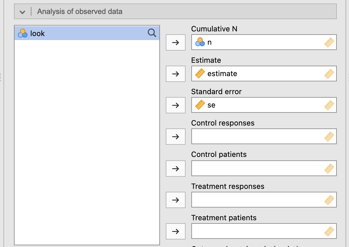
- In the Analysis of observed data box, move n to Cumulative N, estimate to Estimate and se to Standard error.
The Interim analyses table gives P(benefit) = 0.923 after 57 patients (continue) and 0.994 after 114 (stop for efficacy), with the posterior mean shrunk from 0.55 to 0.40. The design tables above it give the sceptical row of Table 2.
References
Berry, Donald A. 2006. “Bayesian Clinical Trials.” Nature Reviews Drug Discovery 5 (1): 27–36. https://doi.org/10.1038/nrd1927.
Grünwald, Peter, Rianne de Heide, and Wouter Koolen. 2024. “Safe Testing.” Journal of the Royal Statistical Society Series B: Statistical Methodology 86 (5): 1091–128. https://doi.org/10.1093/jrsssb/qkae011.
Lee, J Jack, and Diane D Liu. 2008. “A Predictive Probability Design for Phase II Cancer Clinical Trials.” Clinical Trials 5 (2): 93–106. https://doi.org/10.1177/1740774508089279.
Rouder, Jeffrey N. 2014. “Optional Stopping: No Problem for Bayesians.” Psychonomic Bulletin & Review 21 (2): 301–8. https://doi.org/10.3758/s13423-014-0595-4.
Rouder, Jeffrey N., Paul L. Speckman, Dongchu Sun, Richard D. Morey, and Geoffrey Iverson. 2009. “Bayesian t Tests for Accepting and Rejecting the Null Hypothesis.” Psychonomic Bulletin & Review 16 (2): 225–37. https://doi.org/10.3758/pbr.16.2.225.
Ryan, Elizabeth G., Kristian Brock, Simon Gates, and Daniel Slade. 2020. “Do We Need to Adjust for Interim Analyses in a Bayesian Adaptive Trial Design?” BMC Medical Research Methodology 20 (1). https://doi.org/10.1186/s12874-020-01042-7.
Schönbrodt, Felix D., and Eric-Jan Wagenmakers. 2018. “Bayes Factor Design Analysis: Planning for Compelling Evidence.” Psychonomic Bulletin & Review 25 (1): 128–42. https://doi.org/10.3758/s13423-017-1230-y.
Schönbrodt, Felix D., Eric-Jan Wagenmakers, Michael Zehetleitner, and Marco Perugini. 2017. “Sequential Hypothesis Testing with Bayes Factors: Efficiently Testing Mean Differences.” Psychological Methods 22 (2): 322–39. https://doi.org/10.1037/met0000061.
Spiegelhalter, David J., Laurence S. Freedman, and Mahesh K. B. Parmar. 1994. “Bayesian Approaches to Randomized Trials.” Journal of the Royal Statistical Society. Series A (Statistics in Society) 157 (3): 357. https://doi.org/10.2307/2983527.
Stallard, Nigel, Susan Todd, Elizabeth G. Ryan, and Simon Gates. 2020. “Comparison of Bayesian and Frequentist Group-Sequential Clinical Trial Designs.” BMC Medical Research Methodology 20 (1). https://doi.org/10.1186/s12874-019-0892-8.
Stefan, Angelika M., Felix D. Schönbrodt, Nathan J. Evans, and Eric-Jan Wagenmakers. 2022. “Efficiency in Sequential Testing: Comparing the Sequential Probability Ratio Test and the Sequential Bayes Factor Test.” Behavior Research Methods 54 (6): 3100–3117. https://doi.org/10.3758/s13428-021-01754-8.
Thall, Peter F., and Richard Simon. 1994. “Practical Bayesian Guidelines for Phase IIB Clinical Trials.” Biometrics 50 (2): 337. https://doi.org/10.2307/2533377.
U.S. Food and Drug Administration. 2019. Adaptive Designs for Clinical Trials of Drugs and Biologics: Guidance for Industry.