| Stopping look | Proportion of trials | Mean estimate / true effect |
|---|---|---|
| 1 | 0.034 | 2.177 |
| 2 | 0.524 | 1.244 |
| 3 (final) | 0.442 | 0.775 |
| All trials | 1.000 | 1.068 |
Inference after a sequential test
Why the naive estimate, confidence interval and p-value are wrong after early stopping, and the methods that correct them.
The naive analysis is biased
When a trial stops because its \(Z\) statistic crossed a boundary, it has been selected for being extreme. The ordinary estimate at the stopping look is therefore biased away from zero. A confidence interval that ignores the stopping rule has the wrong coverage, and the naive p-value is too small. The bias is largest for trials that stop very early (Bassler et al. 2010; Robertson et al. 2023a).
The simulation below takes the design from Futility’s first example (three looks, O’Brien–Fleming-type efficacy boundary, no futility). It generates 100 000 trials in which the true effect is exactly the design effect \(\theta_1\), and records the naive estimate at the look where each trial stops.
Trials that stop at the first look report, on average, 2.2 times the true effect; those stopping at the second look 1.24 times. Trials that run to the end underestimate it, because the large estimates were removed by early stopping. Across all trials the average bias is modest, but a single trial stopped early should not be taken at face value.
Repeated confidence intervals
Jennison and Turnbull (1989) proposed repeated confidence intervals (RCIs): a sequence of intervals that contains \(\theta\) simultaneously at every look with probability \(1-\alpha\),
\[ \hat\theta_k \pm \frac{c_k}{\sqrt{I_k}}, \]
where \(c_k\) are the boundaries of a two-sided level-\(\alpha\) group sequential test. Because the coverage is simultaneous, an RCI is valid whatever the stopping decision — even if the monitoring committee departs from the boundaries. That makes RCIs the natural interval to report at interim looks. At the final analysis they are conservative.
Exact inference at the end of the trial
For the final report, the sample space of outcomes \((k^*, z^*)\) — stopping look and statistic — must be ordered to define what “more extreme” means. The stagewise ordering ranks outcomes first by how early the efficacy boundary was crossed, then by \(z\) within the same look (Fairbanks and Madsen 1982; Tsiatis et al. 1984):
- p-value. \(P_{H_0}\) of stopping for efficacy earlier than \(k^*\), or at \(k^*\) with a statistic at least \(z^*\).
- Confidence interval. All \(\theta\) for which the same probability, computed under \(\theta\), lies between \(\alpha/2\) and \(1-\alpha/2\).
- Median-unbiased estimate. The \(\theta\) at which that probability is exactly 0.5.
The stagewise ordering depends only on the looks already done: it does not need the future schedule. Its p-value agrees with the test decision. Other orderings (likelihood ratio, maximum likelihood estimate) and bias-adjusted estimators exist, each with its own properties (Emerson and Fleming 1990; Robertson et al. 2023a, 2023b). All of these quantities are computed with the same numerical engine as the boundaries, by solving over \(\theta\).
Reporting
The CONSORT extension for adaptive designs asks for the planned and actual looks, the boundaries, the reason for stopping, and estimates and intervals that account for the design (Dimairo et al. 2020).
Example: the same data under two designs
A trial runs to its final analysis, with \(Z\) = 0.5, 1.0 and 2.4 at information fractions 0.35, 0.72 and 1. The table compares the naive analysis of the final data with the stagewise analysis under an O’Brien–Fleming-type and a Pocock-type design (Lan–DeMets spending, one-sided \(\alpha = 0.025\); effect as a multiple of the design effect).
| Analysis | Estimate | Lower | Upper | p-value |
|---|---|---|---|---|
| Naive (fixed sample) | 0.7360 | 0.1350 | 1.3371 | 0.0082 |
| Stagewise, O’Brien-Fleming type | 0.7094 | 0.0876 | 1.3196 | 0.0129 |
| Stagewise, Pocock type | 0.6795 | 0.0087 | 1.3029 | 0.0237 |
The stagewise analysis accounts for the two earlier chances of stopping. It gives a larger p-value, a smaller median-unbiased estimate and an interval shifted towards zero. The correction is larger under the Pocock-type design, which spent more \(\alpha\) at the interim looks; the naive p-value ignores both. Under the stagewise ordering a trial that stops at its first look gets exactly the fixed-sample analysis: only \(Z_1\) matters there. Estimators that also correct the bias of early stops use other orderings or explicit bias adjustment (Emerson and Fleming 1990; Robertson et al. 2023a).
TipIn jmsequential
Sequential → Group Sequential Design with a dataset (version 0.1.0). When a boundary is crossed, or the last row is marked as the final analysis, the Inference after stopping table gives:
- the naive estimate and confidence interval, for reference;
- the stagewise-ordering median-unbiased estimate and interval;
- the stagewise p-value.
Repeated confidence intervals appear in the Interim analyses table at every look. For one-sided designs these numbers agree with rpact to at least five decimals. For two-sided designs rpact reports the naive estimate and interval instead.
The example in jamovi
The looks of the example go into a small data set: the cumulative N (35 %, 72 % and 100 % of the default design’s 171 patients), Z and the information fraction.
| look | n | z | t |
|---|---|---|---|
| 1 | 60 | 0.50 | 0.35 |
| 2 | 123 | 1.00 | 0.72 |
| 3 | 171 | 2.40 | 1.00 |
- Sequential → Group Sequential Design: the defaults are the O’Brien–Fleming-type design of the example.
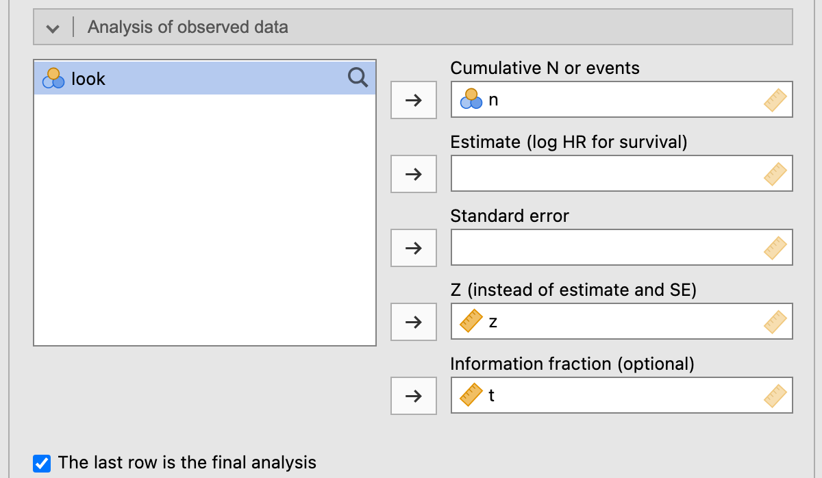
- In the Analysis of observed data box, move n to Cumulative N or events, z to Z (instead of estimate and SE) and t to Information fraction, and tick The last row is the final analysis.
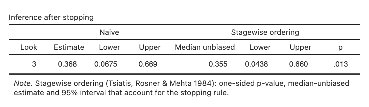
The Inference after stopping table gives the O’Brien–Fleming rows of Table 2 on the scale of the difference in means (the design effect is 0.5): naive estimate 0.368 (95 % CI 0.067–0.669), median-unbiased estimate 0.355 (0.044–0.660) and stagewise p = 0.013.
References
Bassler, Dirk, Matthias Briel, Victor M. Montori, et al. 2010. “Stopping Randomized Trials Early for Benefit and Estimation of Treatment Effects: Systematic Review and Meta-Regression Analysis.” JAMA 303 (12): 1180. https://doi.org/10.1001/jama.2010.310.
Dimairo, Munyaradzi, Philip Pallmann, James Wason, et al. 2020. “The Adaptive Designs CONSORT Extension (ACE) Statement: A Checklist with Explanation and Elaboration Guideline for Reporting Randomised Trials That Use an Adaptive Design.” BMJ, m115. https://doi.org/10.1136/bmj.m115.
Emerson, Scott S., and Thomas R. Fleming. 1990. “Parameter Estimation Following Group Sequential Hypothesis Testing.” Biometrika 77 (4): 875–92. https://doi.org/10.1093/biomet/77.4.875.
Fairbanks, Kenneth, and Richard Madsen. 1982. “P Values for Tests Using a Repeated Significance Test Design.” Biometrika 69 (1): 69–74. https://doi.org/10.1093/biomet/69.1.69.
Jennison, Christopher, and Bruce W. Turnbull. 1989. “Interim Analyses: The Repeated Confidence Interval Approach.” Journal of the Royal Statistical Society Series B: Statistical Methodology 51 (3): 305–34. https://doi.org/10.1111/j.2517-6161.1989.tb01433.x.
Robertson, David S., Babak Choodari‐Oskooei, Munya Dimairo, Laura Flight, Philip Pallmann, and Thomas Jaki. 2023a. “Point Estimation for Adaptive Trial Designs i: A Methodological Review.” Statistics in Medicine 42 (2): 122–45. https://doi.org/10.1002/sim.9605.
Robertson, David S., Babak Choodari‐Oskooei, Munya Dimairo, Laura Flight, Philip Pallmann, and Thomas Jaki. 2023b. “Point Estimation for Adaptive Trial Designs II: Practical Considerations and Guidance.” Statistics in Medicine 42 (14): 2496–520. https://doi.org/10.1002/sim.9734.
Tsiatis, Anastasios A., Gary L. Rosner, and Cyrus R. Mehta. 1984. “Exact Confidence Intervals Following a Group Sequential Test.” Biometrics 40 (3): 797. https://doi.org/10.2307/2530924.