Group sequential designs fix the maximum sample size and the spending of \(\alpha\) in advance. Some settings do not allow that:
Anytime-valid methods control the type I error at any stopping time, however it is chosen (Ramdas et al. 2023).
An e-value is a non-negative statistic \(E\) whose expectation under \(H_0\) is at most 1. By Markov’s inequality, \(P_{H_0}(E \ge 1/\alpha) \le \alpha\). A sequence of e-values that forms a non-negative supermartingale under \(H_0\) — an e-process — satisfies Ville’s inequality:
\[ P_{H_0}\!\left(\exists\, n:\ E_n \ge 1/\alpha\right) \le \alpha . \]
The data can be monitored after every observation and the test rejects the first time \(E_n \ge 1/\alpha\) (20 for \(\alpha = 0.05\)). The type I error stays controlled even if the study continues beyond any planned size. E-values can also be multiplied across independent studies (Vovk and Wang 2021; Grünwald et al. 2024).
Any likelihood ratio against a fixed alternative is an e-process — Wald’s SPRT statistic is one. Averaging the likelihood ratio over a distribution of alternatives keeps the property. For normal data with variance \(\sigma^2\) and a normal mixing distribution with variance \(\tau^2\), this gives Robbins’ mixture likelihood ratio (Robbins 1970):
\[ E_n = \sqrt{\frac{\sigma^2}{\sigma^2 + n\tau^2}}\; \exp\!\left(\frac{n^2\tau^2(\bar x_n - \theta_0)^2}{2\sigma^2(\sigma^2 + n\tau^2)}\right). \]
Its reciprocal gives the always-valid p-value used by several industry A/B-testing platforms (the mixture SPRT, mSPRT) (Johari et al. 2022).
Inverting an e-process gives a confidence sequence: a sequence of intervals that contains \(\theta\) at all sample sizes simultaneously with probability \(1-\alpha\). For the normal mixture above, the interval at sample size \(n\) is
\[ \bar x_n \pm \sqrt{\frac{2\sigma^2(\sigma^2 + n\tau^2)}{n^2\tau^2}\, \ln\!\left(\frac{\sqrt{1 + n\tau^2/\sigma^2}}{\alpha}\right)} . \]
Nonparametric and asymptotic versions exist (Howard et al. 2021; Waudby-Smith et al. 2024).
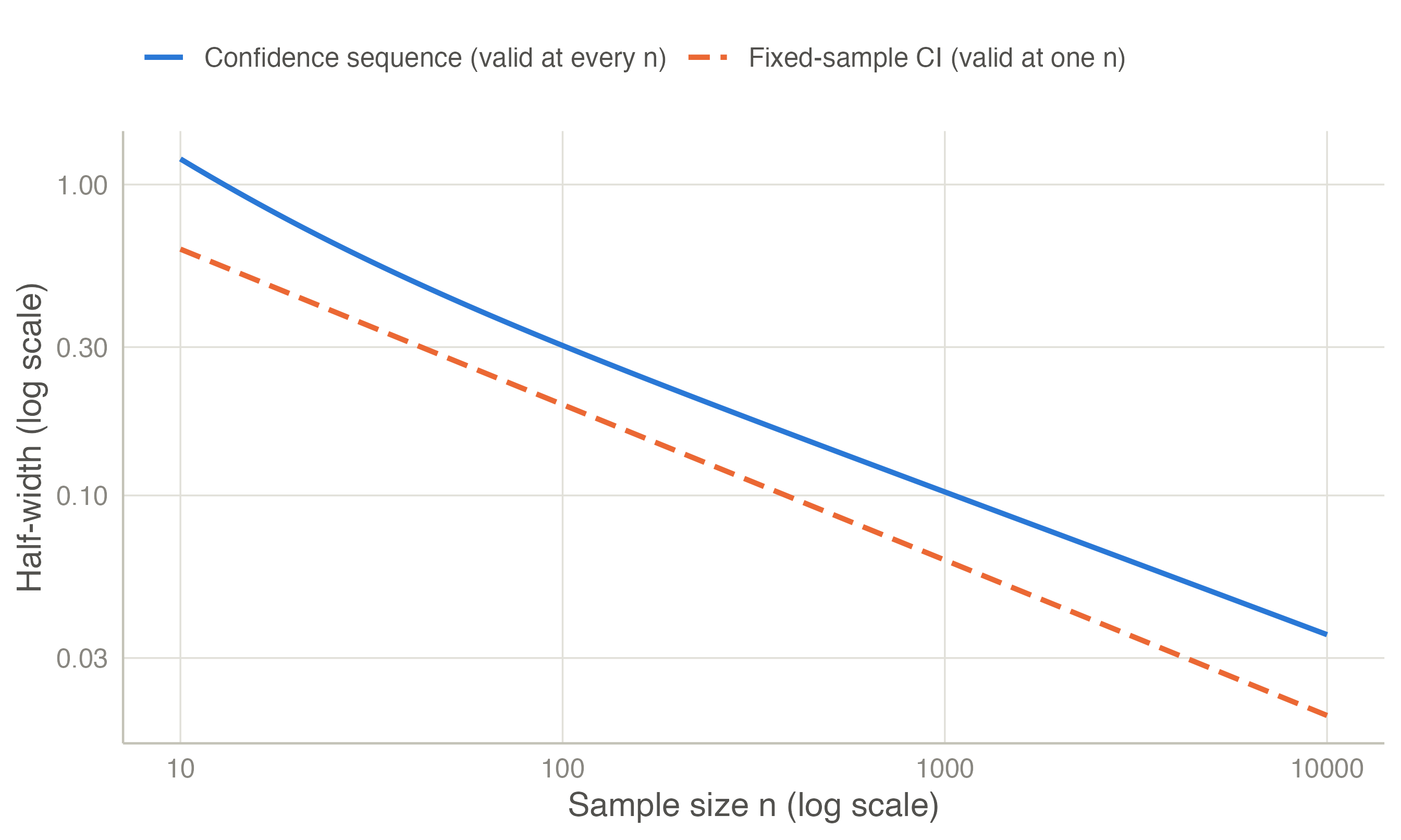
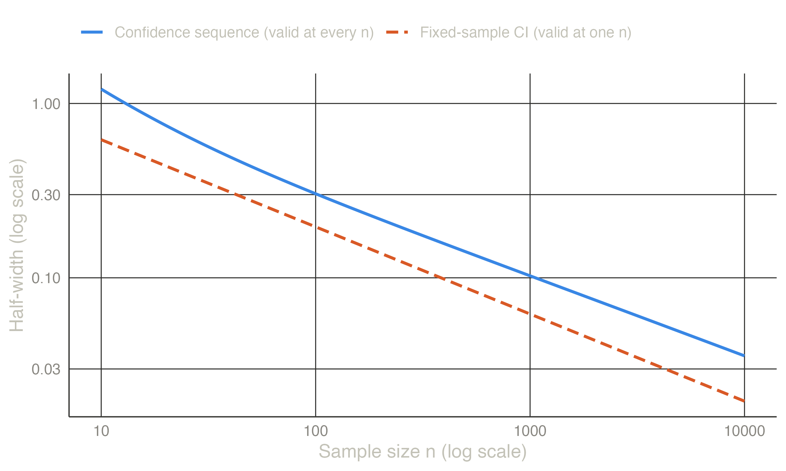
The price of this flexibility is width. A fixed-sample confidence interval is valid only at the one sample size chosen in advance; a confidence sequence is valid at all of them.
At the tuning point \(n = 100\) the confidence sequence is 55 % wider than the fixed interval.
Grünwald et al. (2024) construct safe tests: e-values that grow as fast as possible under the alternative (GROW optimality), for the \(t\)-test, 2×2 tables and other standard settings. An anytime-valid log-rank test exists for survival data (Schure et al. 2024). ALL-IN meta-analysis applies the same ideas to living systematic reviews (Schure and Grünwald 2022).
Compared with a well-planned group sequential design, anytime-valid methods need a somewhat larger sample at a given horizon. In exchange, the analysis plan does not have to be fixed in advance.
The price of anytime validity. Take a one-sample test with known SD, a standardised effect of 0.5, two-sided \(\alpha = 0.05\) and power 80 %. The mixture e-value uses \(g = \delta^2 = 0.25\). The Anytime-Valid Monitoring analysis computes its operating characteristics exactly: with a known SD, “reject when \(E_n \ge 20\)” is a boundary on \(|z_n|\), handled by the same numerical integration as group sequential designs.
| Design | N for 80 % power |
|---|---|
| Fixed-sample z-test, one analysis | 32 |
| The e-value, one analysis | 61 |
| The e-value, tested after every observation | 54 |
Testing after every observation needs 54 patients to reach 80 % power, against 32 for the fixed design. Under the design effect the test usually stops much earlier: the expected sample size is 36.6 and the median 32. The R package safestats estimates the same design by simulation (55 ± 3 patients). For an unknown SD the analysis simulates the safe \(t\)-test. Two samples with \(d = 0.5\) need 218 patients in total for 80 % power with continuous monitoring, against 130 for the fixed-sample \(t\)-test.
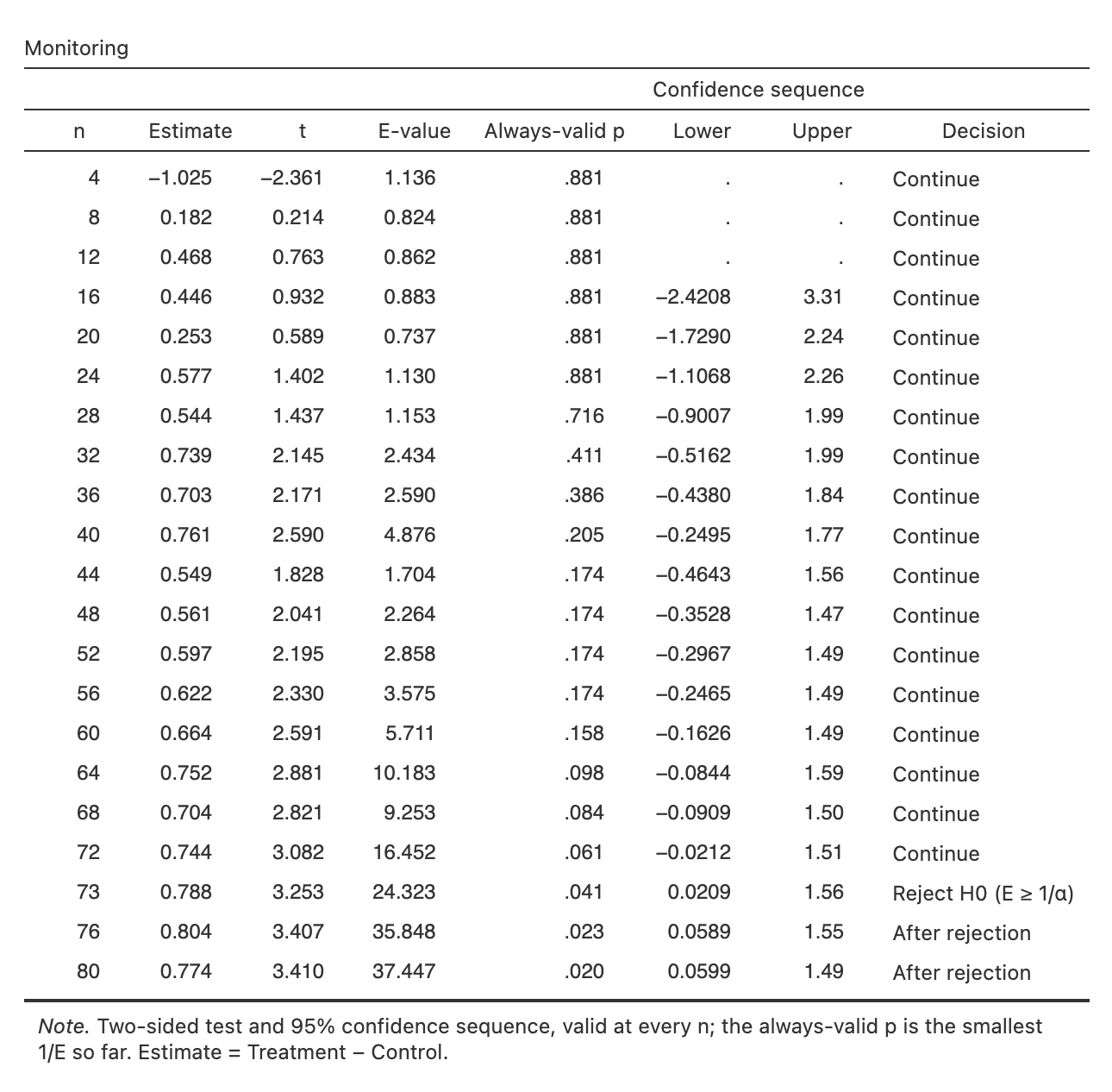
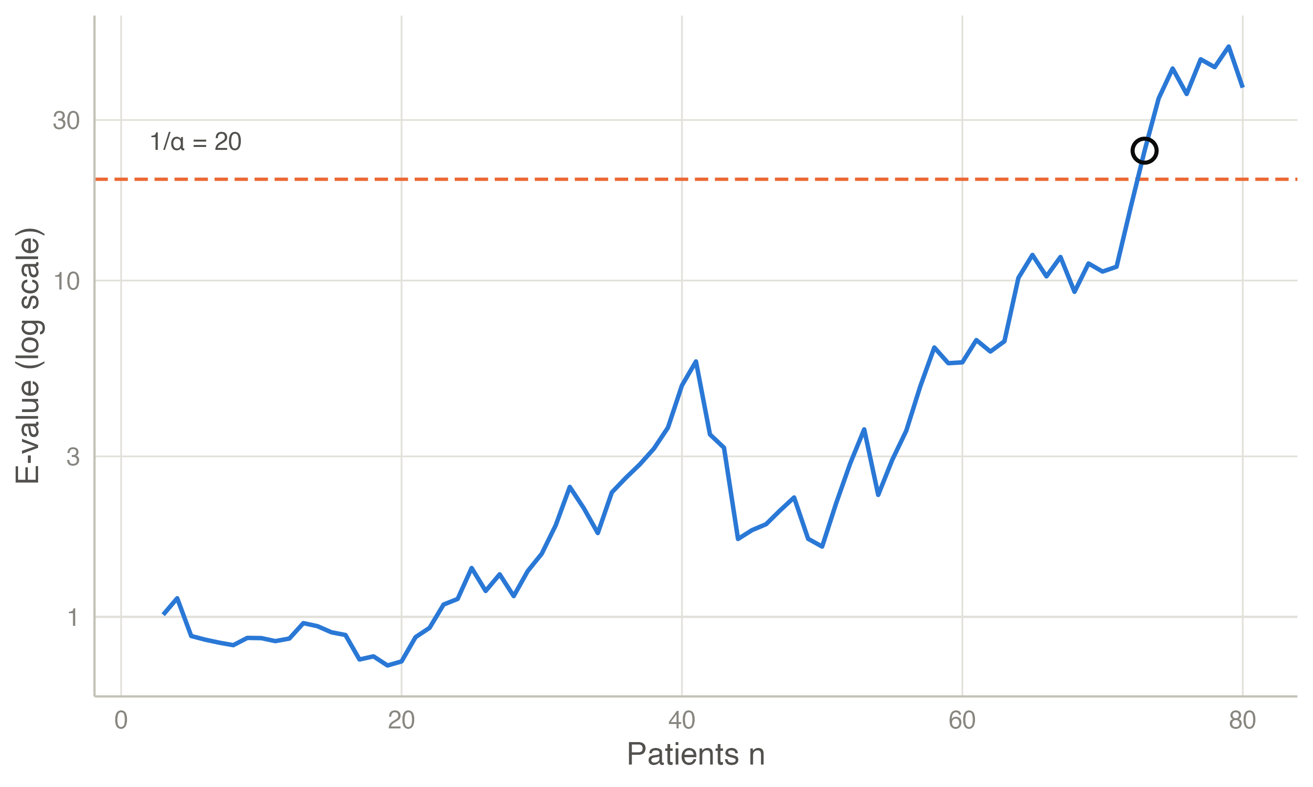
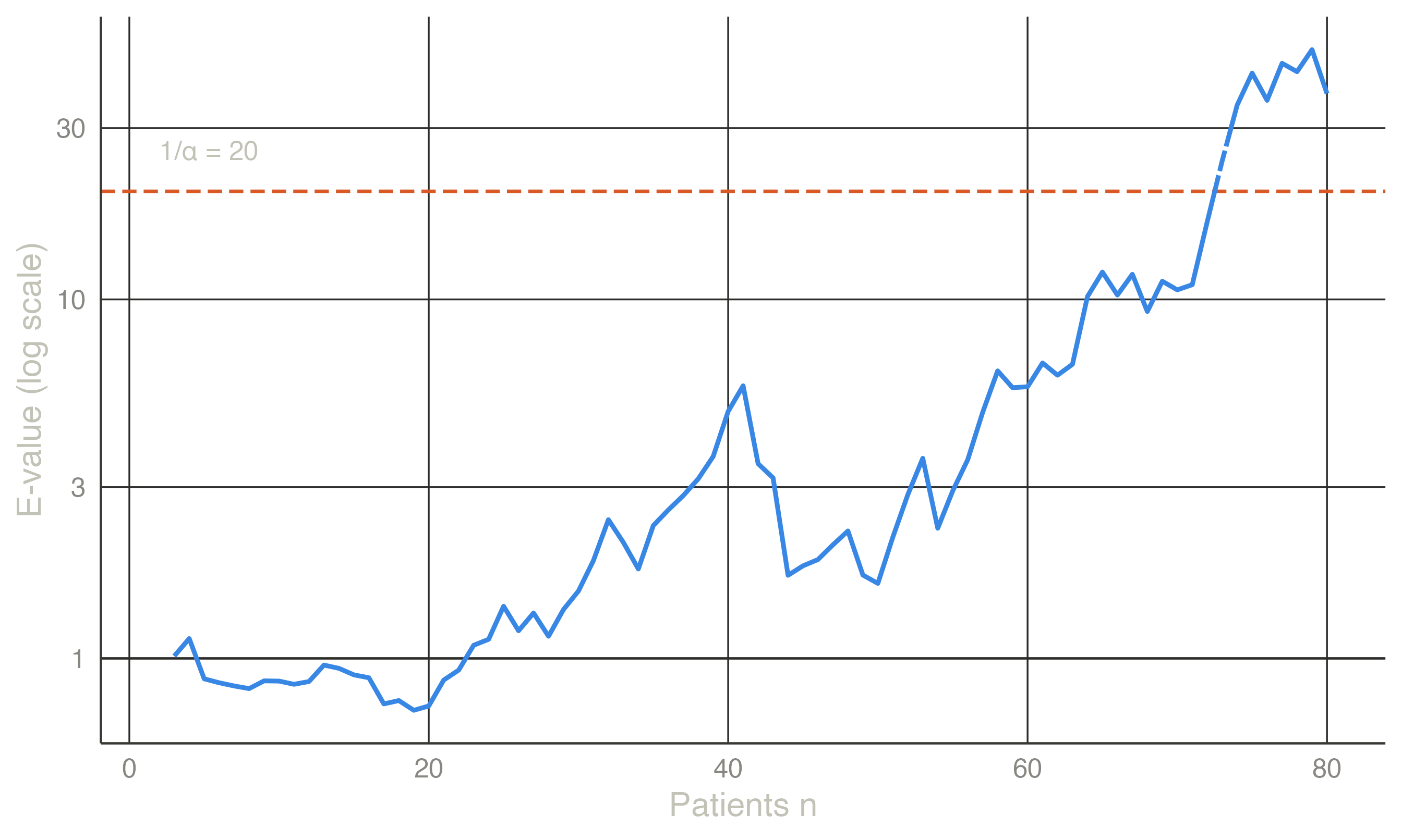
Monitoring. On the dataset Sequential outcomes (80 patients in arrival order, true difference 0.6 SD), the two-sample safe \(t\)-test first reaches \(E \ge 20\) after 73 patients. From then on the 95 % confidence sequence excludes 0. The sequential t-test on the same data stops after 41 patients. It is one-sided, bets on the single alternative \(d = 0.5\), and rejects at a likelihood ratio of \((1-\beta)/\alpha = 16\). The mixture e-value is two-sided and spreads its bet over all effect sizes. That costs speed when the true effect is close to the planned one, and gains robustness when it is not.
Sequential → Anytime-Valid Monitoring (version 0.5.0).
The Monitoring table shows every fourth patient and the decision: E first reaches 1/α = 20 after 73 patients (E = 24.3), and from then on the confidence sequence excludes 0. The Design table above it gives the planned N; the E-process plot further down is Figure 2.