Whitehead’s triangular tests

Straight-line boundaries on the (V, Z) plane, near-optimal expected sample size, and the Christmas-tree correction for discrete looks.

The (V, Z) plane

Whitehead (1997) describes a sequential trial by two statistics:

the efficient score \(Z\), the numerator of the score test (for a difference in means it is proportional to the difference in sums);
its Fisher information \(V\), the null variance of \(Z\).

In the notation of this tutorial, \(V = I\) and \(Z = \hat\theta\, I\), the score statistic \(S\) of Information. The standardised statistic is \(Z/\sqrt V\). Under the canonical distribution, \(Z\) is a Brownian motion in “time” \(V\) with drift \(\theta\). Straight lines on this plane are therefore natural boundaries (Whitehead and Jones 1979; Whitehead 1999).

The triangular test

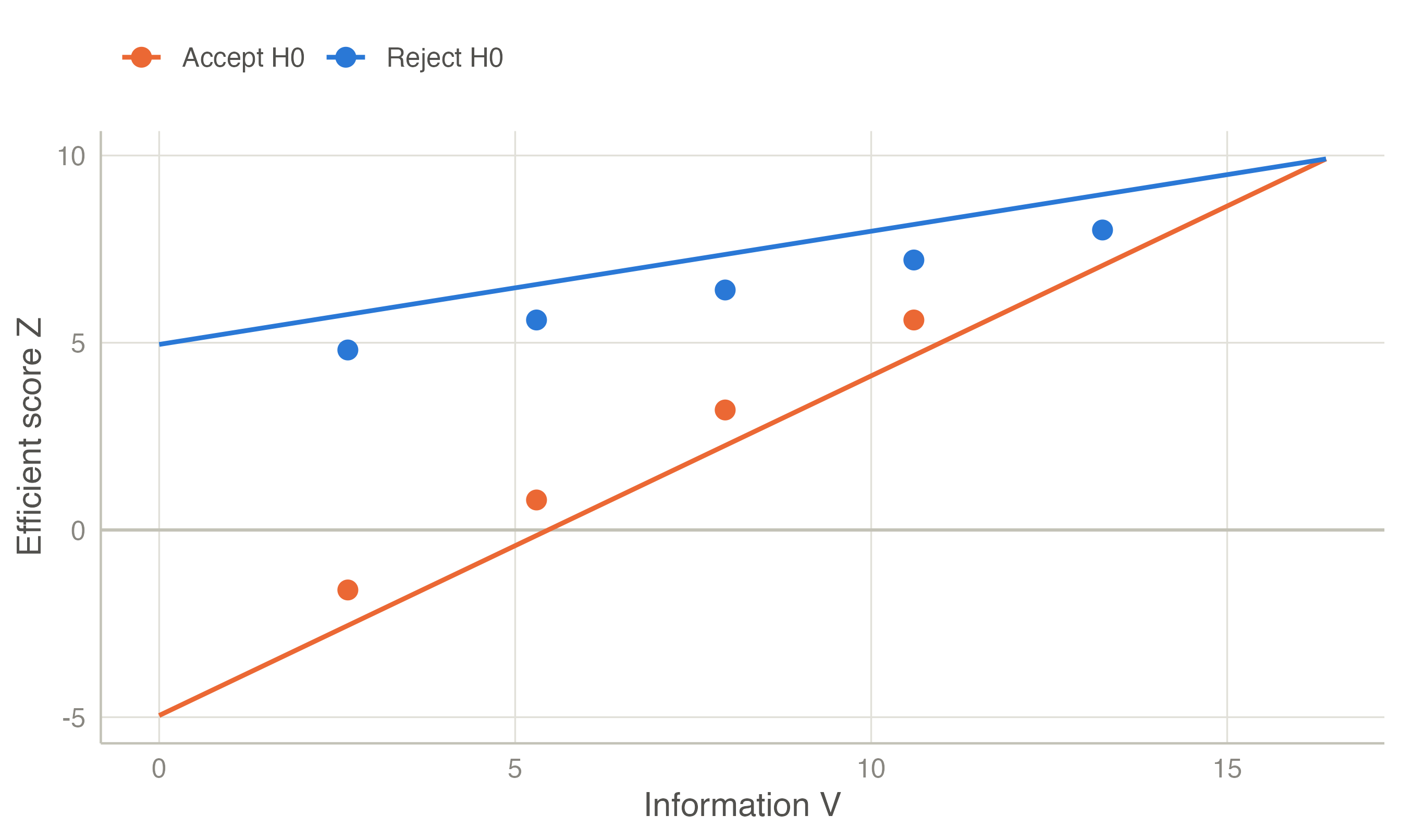
For a one-sided test of \(H_0\!: \theta \le 0\) against \(\theta = \theta_1 > 0\), with type I error \(\alpha\) and power \(1-\beta\), the triangular test continues while

\[ -a + 3cV \;<\; Z \;<\; a + cV , \]

rejecting \(H_0\) above the upper line and accepting it below the lower one. With \(k = 1 + z_{1-\beta}/z_{1-\alpha}\),

\[ a = \frac{k \,\ln\!\big(1/(2\alpha)\big)}{\theta_1}, \qquad c = \frac{\theta_1}{2k}. \]

When \(\alpha = \beta\) these reduce to \(a = 2\ln(1/(2\alpha))/\theta_1\) and \(c = \theta_1/4\). The two lines meet at \(V_{\max} = a/c\), so the test is closed: it can never run beyond \(V_{\max}\). Among tests with the same error rates, it nearly minimises the maximum expected sample size (Whitehead and Stratton 1983; Jennison and Turnbull 2000).

Discrete looks. The formulas assume continuous monitoring. When the data are examined only at looks \(V_1 < V_2 < \dots\), a path can jump over a boundary between looks. The “Christmas-tree” correction pulls both boundaries in by \(0.583\sqrt{V_k - V_{k-1}}\) at look \(k\) (Whitehead 1997). The corrected boundaries therefore meet before the apex of the original triangle. jmsequential chooses the maximum information so that they meet exactly at the last planned look, as SAS PROC SEQDESIGN does, so every planned look can be reached. At that look, \(H_0\) is rejected if \(Z \ge 2cV\).

Two-sided alternative. The double triangular test joins two triangles, one for each sign of \(\theta\), each at level \(\alpha/2\). The region where both close becomes an inner wedge in which the trial stops with “no difference”.

jmsequential computes the boundaries from these formulas, then reports the exact attained \(\alpha\) and power from its numerical engine, because the formulas are approximations.

Figure 1: Triangular test on the (V, Z) plane: continuous boundaries (lines) and the corrected boundaries at 5 looks (points), which meet at the last look. V is in units of 1/θ₁²; α = 0.025, power 90 %.

Example: attained errors and sample size

Table 1: Triangular tests with one-sided alpha = 0.025 and power 90 %: exact attained errors and sample sizes relative to the fixed design.

Design	Attained alpha	Power	Max n	E n \| H0	E n \| H1
Triangular, 5 looks	0.0253	0.9021	1.2609	0.5822	0.6802
Triangular, 10 looks	0.0251	0.9024	1.3418	0.5453	0.6457
Triangular, 20 looks	0.0250	0.9025	1.4022	0.5257	0.6273
LD O’Brien-Fleming, 10 looks	0.0250	0.9000	1.0355	1.0310	0.7223

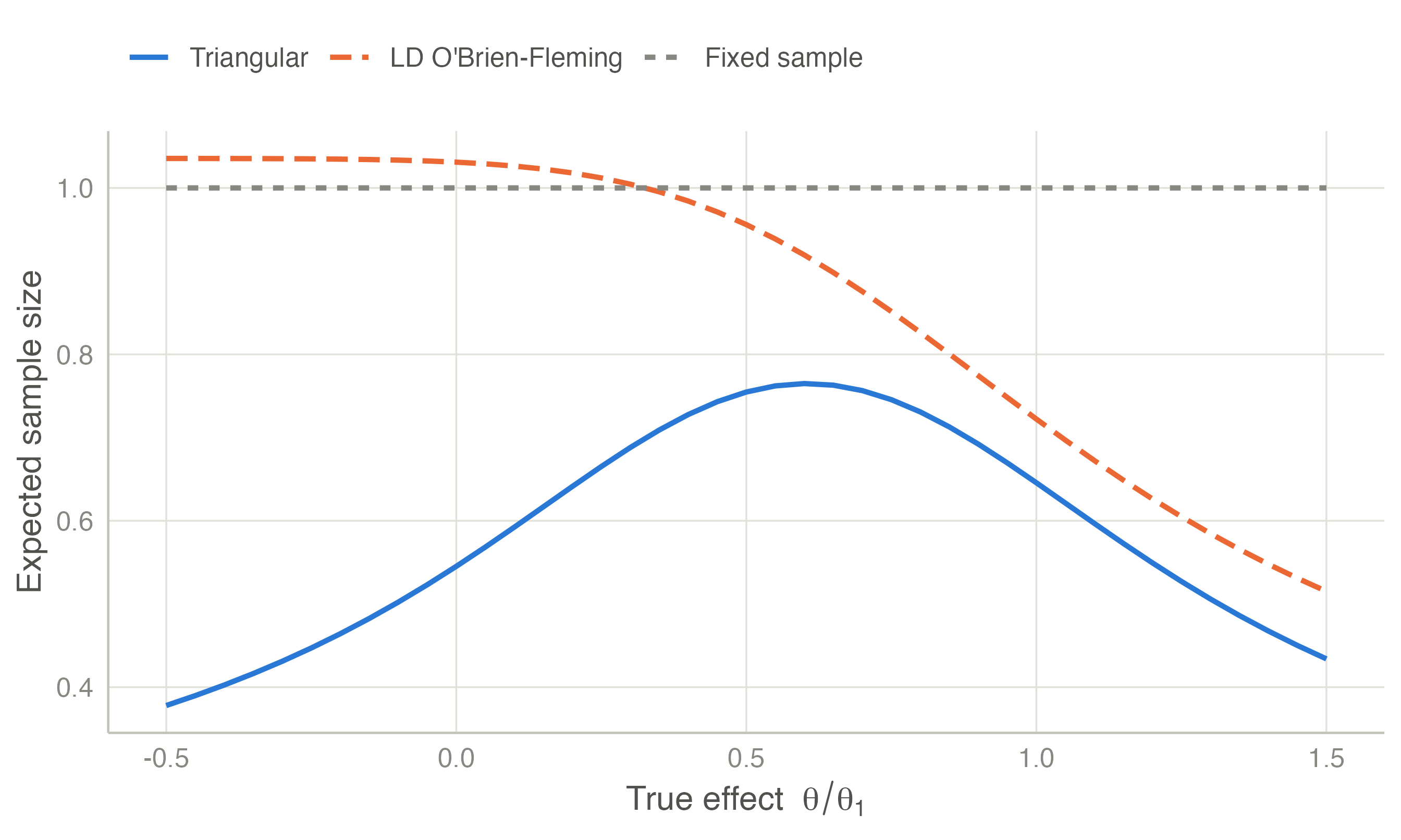
The triangular test needs a larger maximum sample size than O’Brien–Fleming, and more so the more often it looks. In exchange it stops much earlier on average under both hypotheses, especially under \(H_0\), where the O’Brien–Fleming design has no futility boundary. The attained \(\alpha\) and power are close to their targets, and closer as looks become more frequent.

Figure 2: Expected sample size (relative to the fixed design) across true effects, 10 looks.

Triangular tests are available in SAS PROC SEQDESIGN and PEST. In psychology they have been popularised by the R package seqtest (Yanagida 2017).

In jmsequential

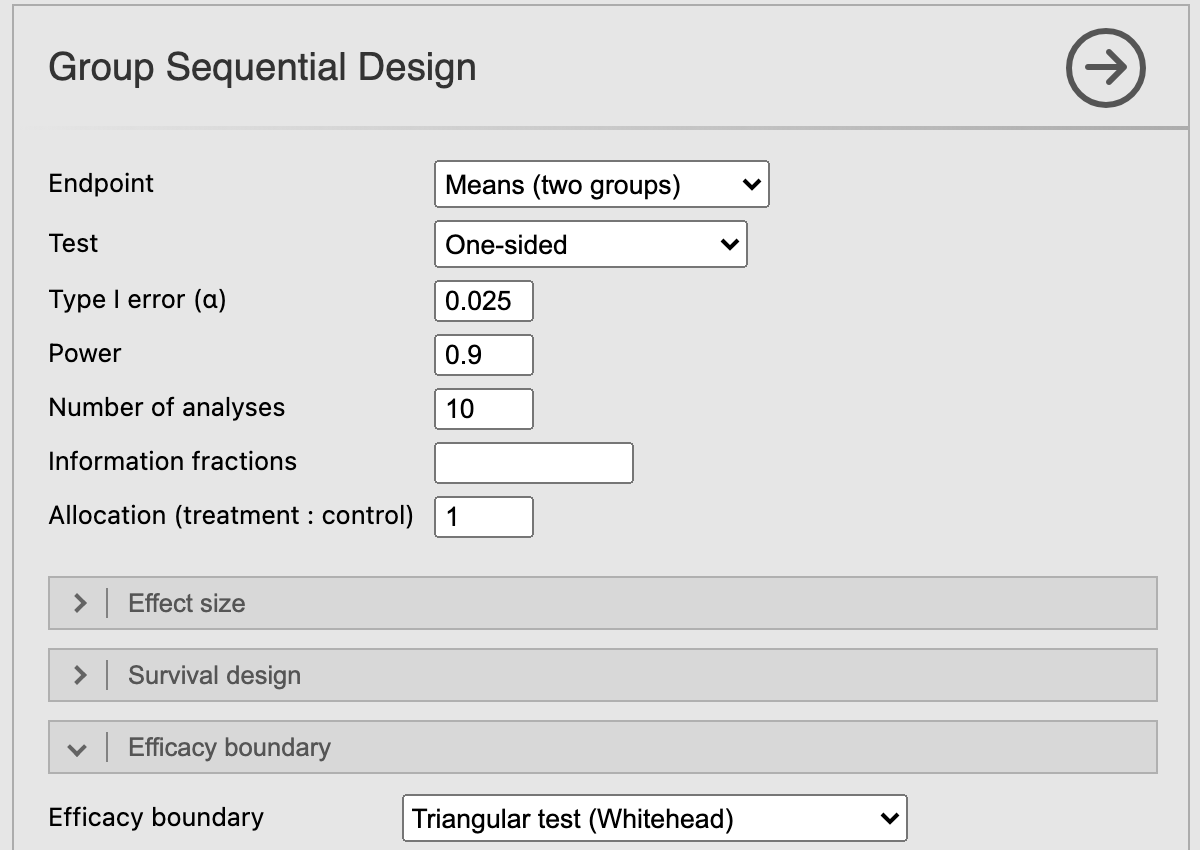
Sequential → Group Sequential Design (from version 0.1.0). Under Efficacy boundary choose Triangular test (Whitehead); two-sided designs give the double triangular test. The results show the exact attained \(\alpha\) and power next to the nominal values. To see the triangle in the boundary plot, set Boundary scale to B-value (Z·√t) and Horizontal axis to Information fraction: the B-value is Whitehead’s score up to a constant, so the boundaries are straight lines. For continuous (observation by observation) triangular monitoring, choose Triangular test (Whitehead, continuous) in the SPRT analysis (from version 0.3.0).

The example in jamovi

Sequential → Group Sequential Design: one-sided α = 0.025 and power 0.9 are the defaults.
Number of analyses: 10.
In the Efficacy boundary box choose Triangular test (Whitehead). Its lower boundary is the test’s own (binding) futility boundary.

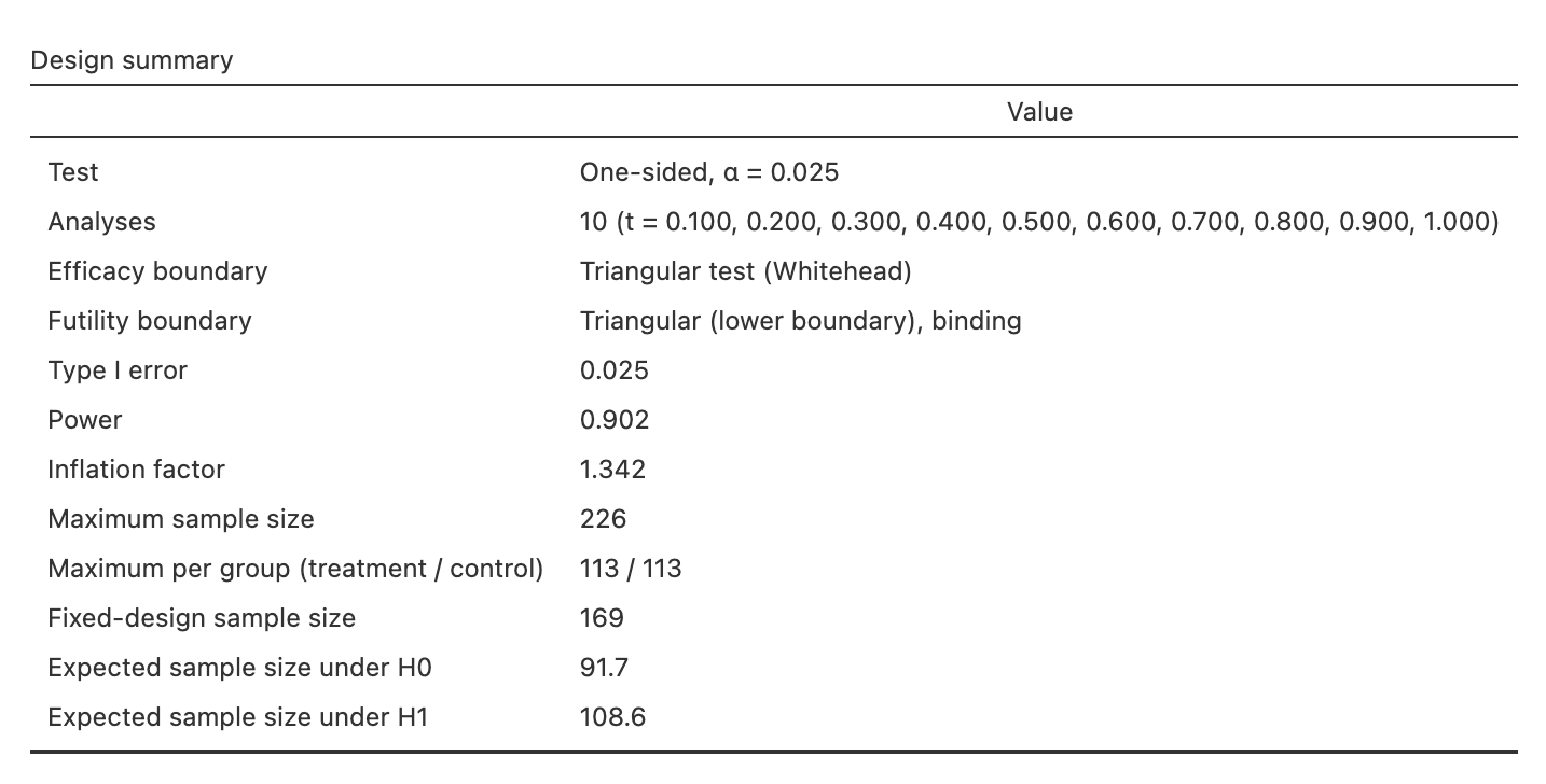
The design summary gives the ten-look row of Table 1 for the default endpoint (a difference in means of 0.5, SD 1): attained α 0.025 and power 0.902, at most 226 patients (inflation factor 1.342) against 169 for a fixed design, and 91.7 and 108.6 patients expected under H0 and H1.

References

Jennison, Christopher, and Bruce Turnbull. 2000. Group Sequential Methods with Applications to Clinical Trials. In Chapman & Hall/CRC Interdisciplinary Statistics Series. Chapman & Hall/CRC. https://doi.org/10.1201/9781584888581.

Whitehead, John. 1997. The Design and Analysis of Sequential Clinical Trials. 2nd revised. Wiley.

Whitehead, John. 1999. “A Unified Theory for Sequential Clinical Trials.” Statistics in Medicine 18 (17-18): 2271–86. https://doi.org/10.1002/(sici)1097-0258(19990915/30)18:17/18<2271::aid-sim254>3.0.co;2-z.

Whitehead, John, and David Jones. 1979. “The Analysis of Sequential Clinical Trials.” Biometrika 66 (3): 443–52. https://doi.org/10.1093/biomet/66.3.443.

Whitehead, John, and Irene Stratton. 1983. “Group Sequential Clinical Trials with Triangular Continuation Regions.” Biometrics 39 (1): 227. https://doi.org/10.2307/2530822.

Yanagida, Takuya. 2017. “Seqtest: An r Package for Sequential Triangular Tests.” Journal of Statistical Theory and Practice 11 (3): 402–6. https://doi.org/10.1080/15598608.2016.1268549.