Classical boundaries need the number and timing of the looks in advance. Real monitoring committees meet when they meet: an analysis may be brought forward because of a safety signal, events may accrue more slowly than planned, an extra look may be added. Lan and DeMets (1983) proposed to plan instead how fast the type I error is used up as information accumulates.
An alpha-spending function \(\alpha(t)\) is non-decreasing on \([0, 1]\), with \(\alpha(0) = 0\) and \(\alpha(1) = \alpha\). It gives the cumulative type I error that may have been spent by information fraction \(t\). At each actual look \(k\), the boundary \(b_k\) is solved so that the probability of crossing it for the first time at that look is exactly the increment
\[ P_{H_0}\!\left(Z_1 < b_1, \dots, Z_{k-1} < b_{k-1},\ Z_k \ge b_k\right) = \alpha(t_k) - \alpha(t_{k-1}). \]
The boundary at a look depends only on the looks already done, so the number and timing of future looks may change freely (provided the changes do not depend on the observed results) (Lan and DeMets 1989; DeMets and Lan 1994). At the final analysis all the remaining \(\alpha\) is spent, even if the information turns out larger or smaller than planned.
jmsequential applies the spending function to the level of one tail: \(\alpha\) for a one-sided design, and \(\alpha/2\) in each tail of a symmetric two-sided design. This is the gsDesign and rpact convention, and it reproduces the published Lan–DeMets tables.
| Function | Cumulative \(\alpha(t)\) | Parameter | Behaves like |
|---|---|---|---|
| Lan–DeMets O’Brien–Fleming type (Lan and DeMets 1983) | \(2 - 2\Phi\!\left(z_{1-\alpha/2}/\sqrt{t}\right)\) | — | O’Brien–Fleming |
| Lan–DeMets Pocock type (Lan and DeMets 1983) | \(\alpha \ln\!\left(1 + (e - 1)t\right)\) | — | Pocock |
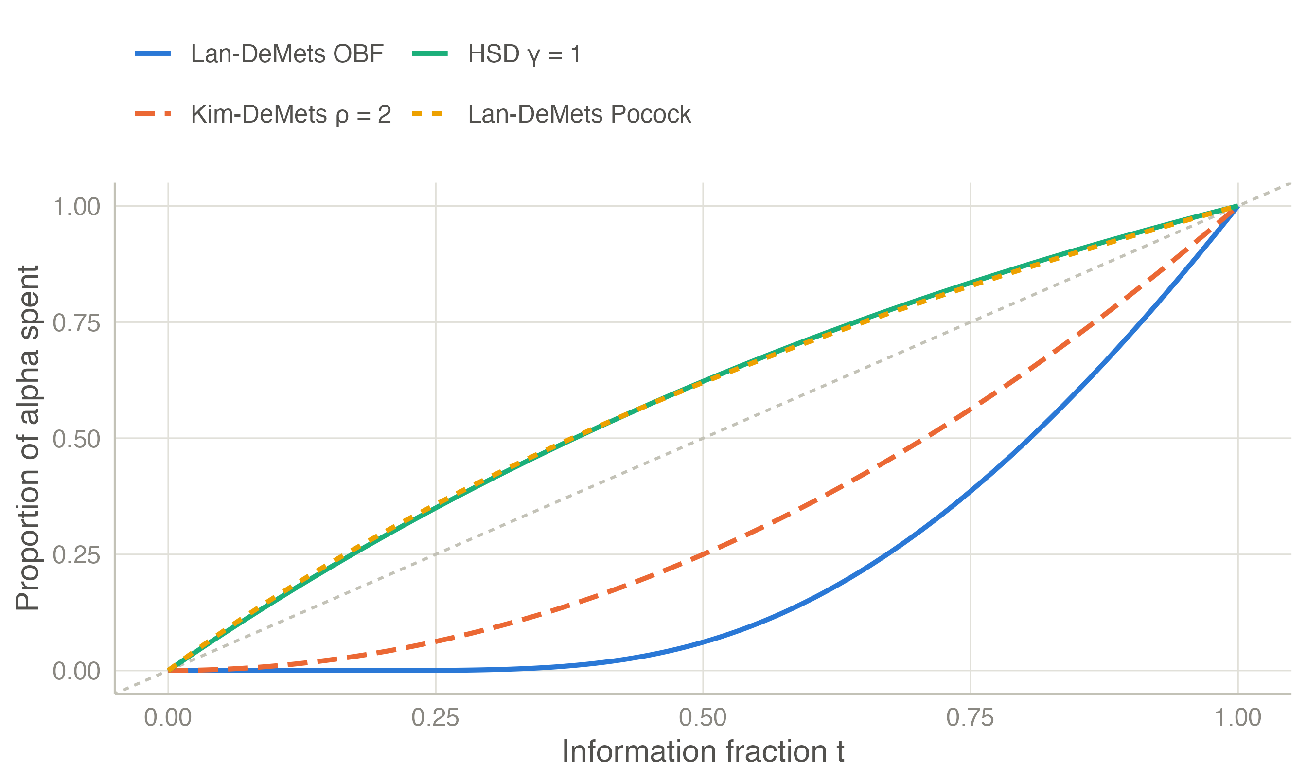
| Kim–DeMets power family (Kim and DeMets 1987) | \(\alpha\, t^{\rho}\) | \(\rho > 0\) | \(\rho = 1\) Pocock-like, \(\rho = 3\) O’Brien–Fleming-like |
| Hwang–Shih–DeCani (Hwang et al. 1990) | \(\alpha \dfrac{1 - e^{-\gamma t}}{1 - e^{-\gamma}}\) | \(\gamma \ne 0\) | \(\gamma = 1\) Pocock-like, \(\gamma = -4\) O’Brien–Fleming-like |
| Exponential (Anderson and Clark 2010) | \(\alpha^{\,t^{-\nu}}\) | \(\nu > 0\) | \(\nu = 0.75\) O’Brien–Fleming-like |
| User-defined | cumulative proportions at the planned looks | — | anything, e.g. Haybittle–Peto-like |
Functions that stay near zero early (O’Brien–Fleming type) keep almost all of \(\alpha\) for the final analysis. Those that rise quickly (Pocock type) make early stopping easier at the price of a stricter final test.
| Look | O’Brien-Fleming | LD O’Brien-Fleming type | Pocock | LD Pocock type |
|---|---|---|---|---|
| 1 | 4.562 | 4.877 | 2.413 | 2.438 |
| 2 | 3.226 | 3.357 | 2.413 | 2.427 |
| 3 | 2.634 | 2.680 | 2.413 | 2.410 |
| 4 | 2.281 | 2.290 | 2.413 | 2.397 |
| 5 | 2.040 | 2.031 | 2.413 | 2.386 |
The Lan–DeMets O’Brien–Fleming-type values in the second column (4.877, 3.357, 2.680, 2.290, 2.031) are the classic published ones.
A trial is planned with three equally spaced looks and Lan–DeMets O’Brien–Fleming-type spending, one-sided \(\alpha = 0.025\), power 90 %. The first interim analysis actually takes place at 40 % of the information and the second at 75 %.
| Look | Planned t | Planned b | Cumulative alpha (planned) | Actual t | Actual b | Cumulative alpha (actual) |
|---|---|---|---|---|---|---|
| 1 | 0.3333 | 3.7103 | 0.0001 | 0.4000 | 3.3569 | 0.0004 |
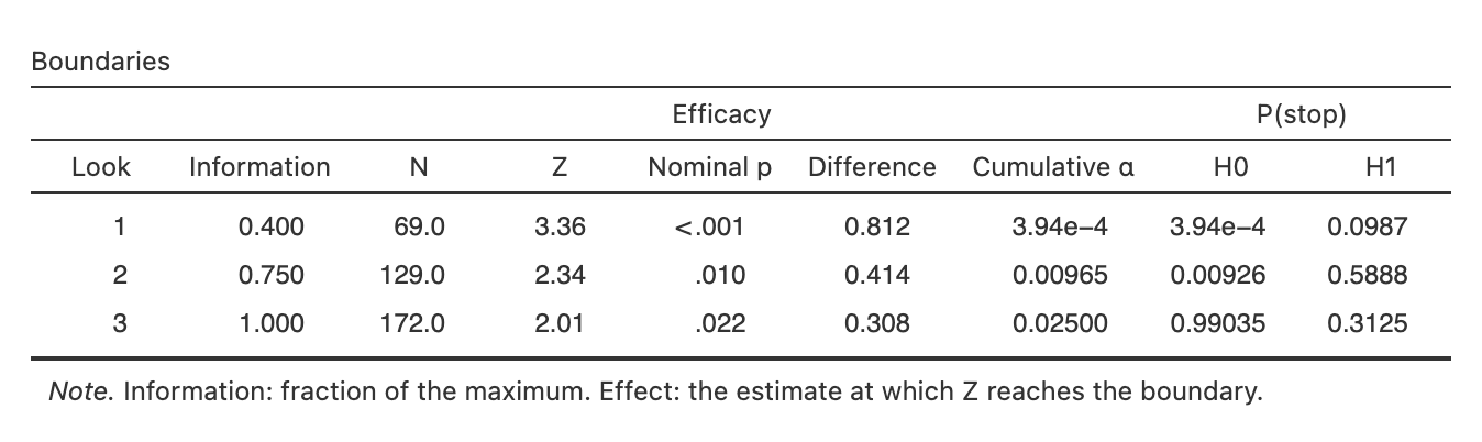
| 2 | 0.6667 | 2.5114 | 0.0060 | 0.7500 | 2.3449 | 0.0096 |
| 3 | 1.0000 | 1.9930 | 0.0250 | 1.0000 | 2.0125 | 0.0250 |
The boundaries adapt to the actual information fractions. The later first look spends more \(\alpha\) and so gets a lower boundary. The total is still exactly 0.025.
Changing the timing is legitimate only if the decision does not depend on the interim results. Otherwise the type I error can be inflated even with a spending function (2006). The spending function itself must be fixed in the protocol.
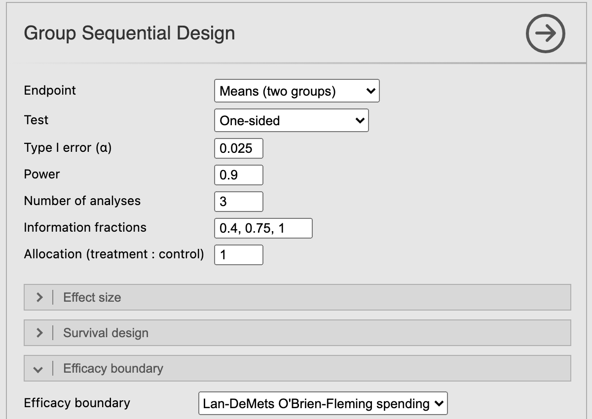
Sequential → Group Sequential Design (from version 0.1.0). Under Efficacy boundary, choose a spending function and its parameter. Enter unequal timings in Information fractions, e.g. 0.4, 0.75, 1 (cumulative sample sizes such as 120, 225, 300 work too). When monitoring (from 0.2.0), the boundaries are recomputed at the information actually observed at each look.
0.4, 0.75, 1 in Information fractions.The Boundaries table gives the actual boundaries of Table 2, 3.36, 2.35 and 2.01, with a cumulative α of 0.0004, 0.0097 and 0.025.