| Look | t | Patients per arm (means) | Events (survival) |
|---|---|---|---|
| 1 | 0.333 | 30 | 118 |
| 2 | 0.667 | 60 | 235 |
| 3 | 1.000 | 90 | 353 |
From information to sample size
Converting a design’s maximum information into patients or events, including survival designs with accrual, follow-up and dropout.
One design, any endpoint
A group sequential design is solved on the \(Z\) scale (Information). Its output is the drift \(\eta = \theta_1\sqrt{I_{\max}}\) that gives the required power, so the maximum information is
\[ I_{\max} = \left(\frac{\eta}{\theta_1}\right)^2 = R \cdot I_{\text{fix}}, \]
where \(R\) is the inflation factor. The endpoint only enters when \(I\) is translated into observations. At look \(k\) the study needs \(t_k\) times the maximum.
Continuous and binary endpoints
With total sample size \(N\), allocation ratio \(r\) (treatment : control) and standard deviation \(\sigma\):
| Endpoint | Information | Maximum sample size |
|---|---|---|
| Two-sample means | \(\dfrac{N r}{(1+r)^2\sigma^2}\) | \(N = I_{\max}\,\sigma^2 (1+r)^2 / r\) |
| One-sample or paired mean | \(n/\sigma^2\) | \(n = I_{\max}\,\sigma^2\) |
| Two proportions (risk difference) | \(\left[\dfrac{1+r}{N}\left(\dfrac{p_1(1-p_1)}{r} + p_0(1-p_0)\right)\right]^{-1}\) | \(N = I_{\max}(1+r)\left(\dfrac{p_1(1-p_1)}{r} + p_0(1-p_0)\right)\) |
Several variance choices are in use for proportions (pooled under \(H_0\), unpooled under \(H_1\), or a mixture). Programs differ slightly for this reason, and each documents its choice.
Time-to-event endpoints
For survival outcomes, information is carried by events, not patients. With allocation \(r:1\) and a log-rank test, Schoenfeld (1983) gives
\[ D = I_{\max}\,\frac{(1+r)^2}{r} = \frac{\eta^2 (1+r)^2}{r\,(\ln \mathrm{HR})^2} \]
events. Freedman (1982) proposed the alternative \(D = \eta^2 (1 + r\,\mathrm{HR})^2 / \{r(1-\mathrm{HR})^2\}\). The analyses are scheduled after \(t_k D\) events.
How many patients give \(D\) events, and when each look happens, depend on accrual, follow-up and dropout. With exponential survival (hazard \(\lambda\)), exponential dropout (hazard \(\gamma\)), uniform accrual over a period \(A\) and a minimum follow-up \(F\), the probability that a patient’s event is observed by the end of the study is
\[ P(\text{event}) = \frac{\lambda}{\lambda+\gamma}\left[1 - \frac{e^{-(\lambda+\gamma)F} - e^{-(\lambda+\gamma)(A+F)}}{(\lambda+\gamma)A}\right], \]
averaged over the arms according to the allocation. Then \(N = D / P(\text{event})\) (Lachin and Foulkes 1986; Lakatos 1988). The expected number of events by calendar time \(\tau\) follows from the same integral truncated at \(\tau\). Solving \(E[D(\tau_k)] = t_k D\) gives the expected calendar time of each look (Kim and Tsiatis 1990). The same model can instead be solved for the accrual duration (given a rate) or for the follow-up (given \(N\)).
Example: two designs from the same boundaries
The design from Futility: one-sided \(\alpha = 0.025\), power 90 %, three looks, Lan–DeMets O’Brien–Fleming-type efficacy and HSD(\(-2\)) non-binding futility.
The fixed-sample equivalents are 85 patients per arm and 331 events. The sequential design needs at most 90 patients per arm (or 353 events), 6.7 % more, and expects to stop well before that when the treatment works or when it clearly does not.
Example: a survival design with accrual, follow-up and dropout
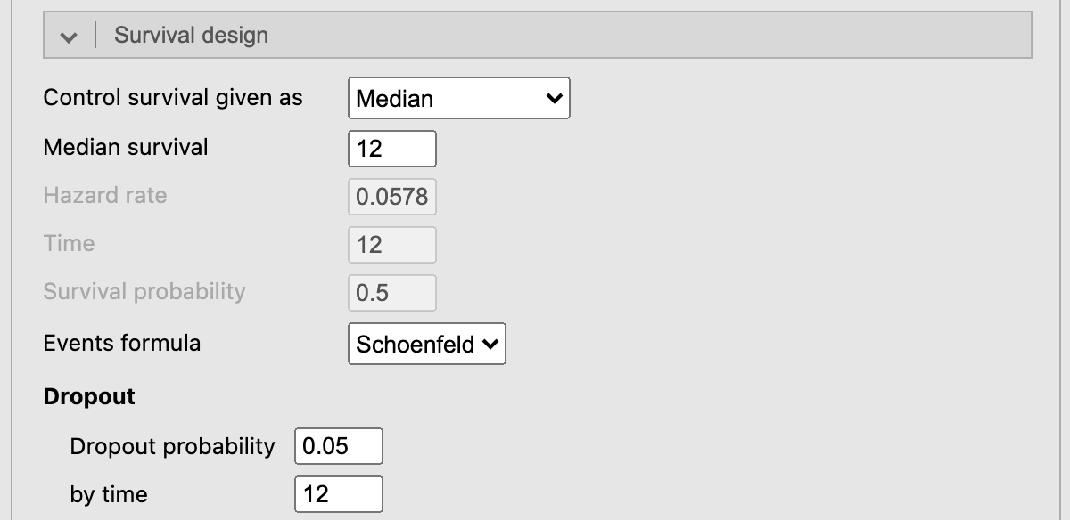
Same boundaries, now for a hazard ratio of 0.7 with a control median of 12 months. Patients are recruited uniformly over 24 months and followed for at least 12 more, and 5 % drop out per year. These are exactly the settings of the example below, computed by the Group Sequential Design analysis itself.
| Look | Events | Months (H1) | Months (H0) | Enrolled (H1) |
|---|---|---|---|---|
| 1 | 118 | 16.6 | 15.4 | 382 |
| 2 | 235 | 25.1 | 23.3 | 551 |
| 3 | 353 | 36.0 | 32.2 | 551 |
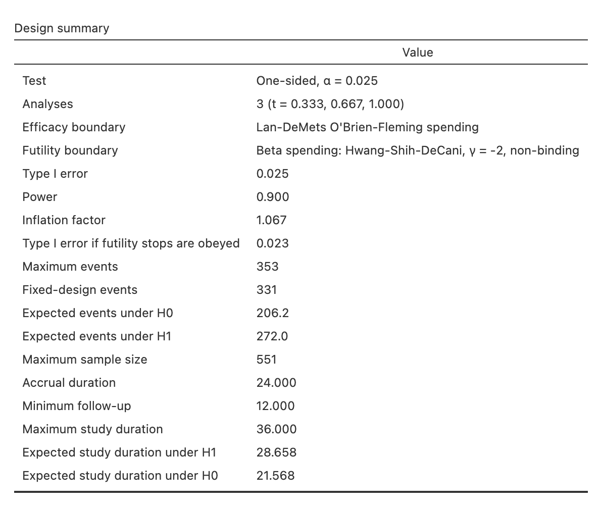
The trial needs 353 events from 551 patients, and lasts at most 36 months. If the treatment works as assumed it is expected to end after 28.7 months; under \(H_0\), thanks to the futility boundary, after 21.6 months. These numbers agree with rpact to within \(10^{-6}\) (relative).
TipIn jmsequential
Sequential → Group Sequential Design (from version 0.1.0).
- Endpoint: means, proportions, time to event, or generic (an effect and the SD of one observation).
- Effect size panel: the hazard ratio for time to event.
- Survival design panel:
- the control survival, as a median, a hazard rate or the survival at a time;
- the events formula;
- dropout;
- what to Calculate: the sample size (accrual duration and minimum follow-up given), the accrual duration (accrual rate and follow-up given), or the follow-up (sample size and accrual given).
The Timing of the analyses table gives the expected calendar time of each look, as above. Accrual is uniform in this version.
The example in jamovi
- Sequential → Group Sequential Design, Endpoint: Time to event. The hazard ratio, in the Effect size box, is 0.7 by default.
- In the Survival design box the defaults are those of the example: control median 12, accrual over 24 and minimum follow-up 12, calculating the sample size. Set Dropout probability to 0.05 by time 12.
- In the Futility boundary box choose Beta spending (Hwang–Shih–DeCani, γ = −2).
The design summary gives 353 events from 551 patients, at most 36 months, and expected durations of 28.7 months under H1 and 21.6 under H0. The Timing of the analyses table, further down, is Table 2.
References
Freedman, L. S. 1982. “Tables of the Number of Patients Required in Clinical Trials Using the Logrank Test.” Statistics in Medicine 1 (2): 121–29. https://doi.org/10.1002/sim.4780010204.
Kim, Kyungmann, and Anastasios A. Tsiatis. 1990. “Study Duration for Clinical Trials with Survival Response and Early Stopping Rule.” Biometrics 46 (1): 81. https://doi.org/10.2307/2531632.
Lachin, John M., and Mary A. Foulkes. 1986. “Evaluation of Sample Size and Power for Analyses of Survival with Allowance for Nonuniform Patient Entry, Losses to Follow-up, Noncompliance, and Stratification.” Biometrics 42 (3): 507. https://doi.org/10.2307/2531201.
Lakatos, Edward. 1988. “Sample Sizes Based on the Log-Rank Statistic in Complex Clinical Trials.” Biometrics 44 (1): 229. https://doi.org/10.2307/2531910.
Schoenfeld, David A. 1983. “Sample-Size Formula for the Proportional-Hazards Regression Model.” Biometrics 39 (2): 499. https://doi.org/10.2307/2531021.