Kaplan-Meier in jamovi

Survival of the whole cohort, median follow-up, survival by performance status, the tests and the plots, from the jamovi panel to the sentence in the paper.

Question. In advanced lung cancer, how long do patients survive, and does survival depend on performance status (ECOG) at enrolment?

Step 0: open the data

Open lung.omv in jamovi. The Variables tab lists the variables, with an icon for each measure type (Figure 1): time and age must be Continuous (ruler), event and sex Nominal (circles), and ecog Ordinal (bars). Double-click a variable to see its setup; the levels of ecog must be in the order ECOG 0, ECOG 1, ECOG 2.

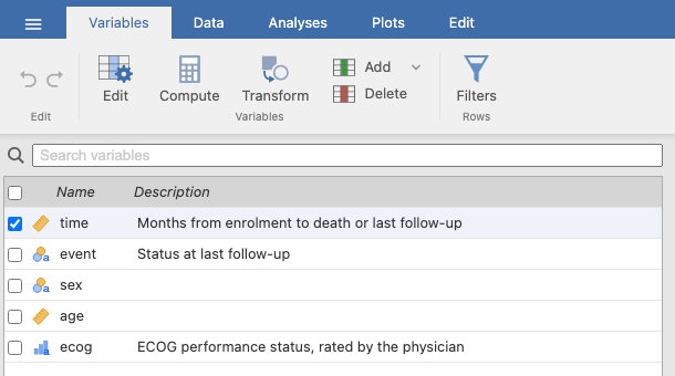
Figure 1: The Variables tab of jamovi with lung.omv open.

The module needs the event as a nominal (or ordinal) variable and asks which of its levels is the event. A column coded 0/1 works once you set its measure type to Nominal. Until you pick the level, the analysis shows nothing, on purpose: guessing which code means “event” is a classic source of errors (in the original lung data, 1 means censored and 2 means dead).

Step 1: the whole cohort

Open Analyses → Prognosis → Kaplan-Meier and set:

Panel	Setting
Time	`time`
Event	`event`; Event level `dead`
Tables → Survival at times	`6, 12, 24`
Tables → Time unit	months
Show on plots	Confidence bands

jamovi syntax

all <- prognosis::km(data = lung, elapsed = time, event = event, eventLevel = "dead",
                     timeUnit = "months", survTimes = "6, 12, 24", ci = TRUE)

Survival summary

				95% CI
N	Events	Censored	Median	Lower	Upper
226	163	63	10.2	9.36	11.9

Survival at given times

				95% CI
Time	At risk	Events	Survival	Lower	Upper
6.00	156	64	71.4 %	65.8 %	77.6 %
12.00	65	119	41.3 %	34.8 %	49.0 %
24.00	13	157	11.7 %	7.2 %	18.8 %

Median survival was 10.18 months (95% CI 9.36–11.93). Survival was 41% at one year and 12% at two years; only 13 patients were still under observation at 24 months, which is why that CI is wide relative to the estimate.

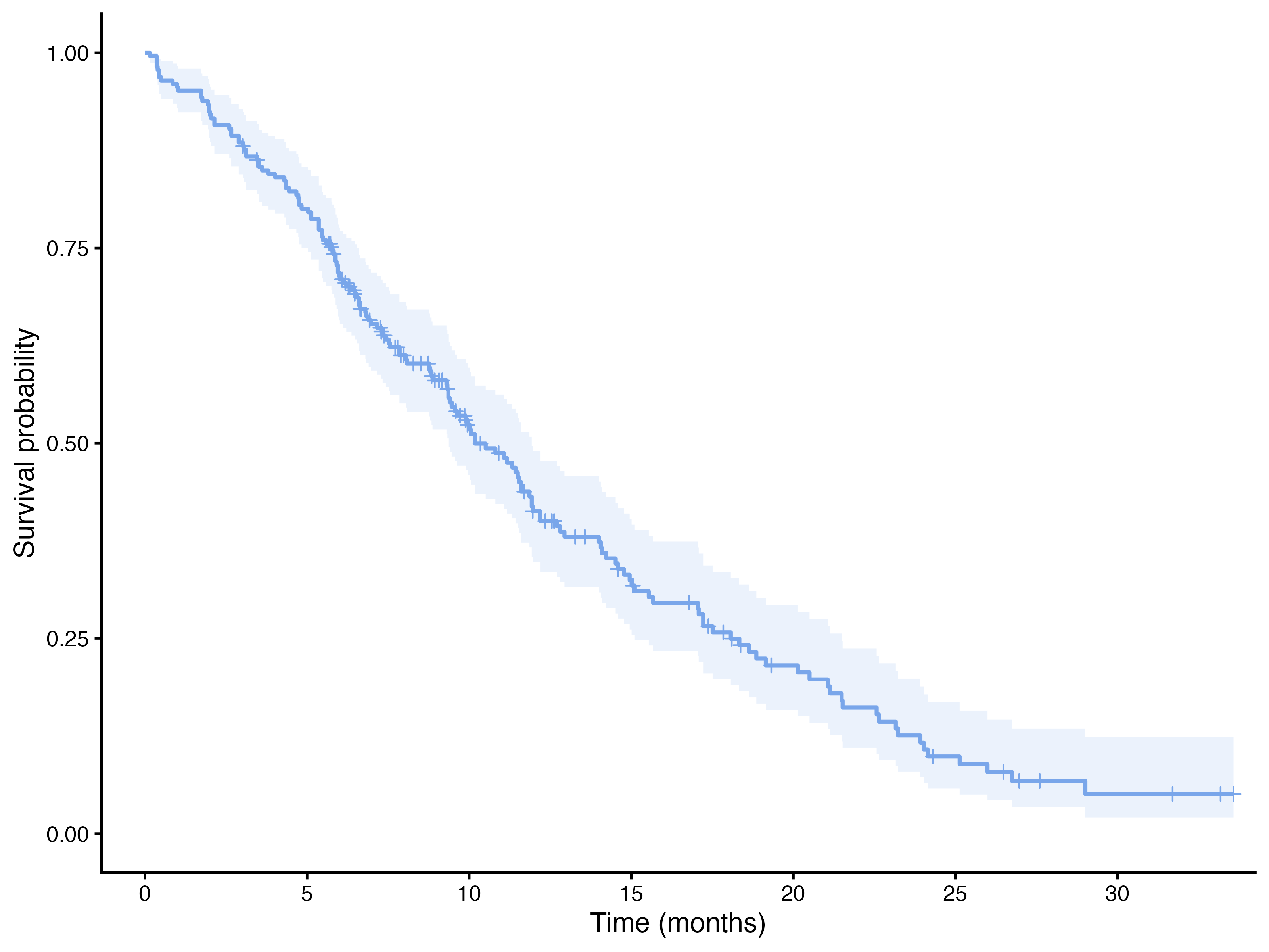
Figure 2: The survival curve of the whole cohort with its 95% confidence band. Crosses mark censored patients.

Median follow-up

A paper should say how long patients were followed. The median of the observed times (8.62 months) underestimates follow-up, because patients who died stop contributing time early. The usual method is the reverse Kaplan-Meier: swap the roles of event and censoring, so that “being censored” is the event. In the module, simply choose alive as the event level:

jamovi syntax

revkm <- prognosis::km(data = lung, elapsed = time, event = event, eventLevel = "alive",
                     kmPlot = FALSE)

Survival summary

				95% CI
N	Events	Censored	Median	Lower	Upper
226	63	163	19.3	16.8	33.2

The median follow-up was 19.32 months (95% CI 16.79–33.18). Change the event level back to dead before going on.

Step 2: survival by ECOG

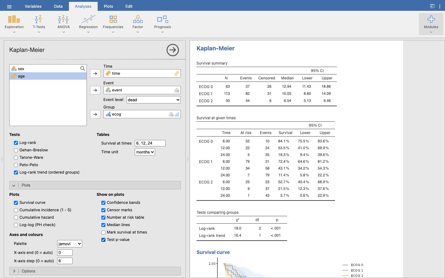
Add ecog to Group, and set:

Panel	Setting
Tests	Log-rank; Log-rank trend (ordered groups)
Show on plots	Confidence bands, Number at risk table, Median lines, Test p-value
Axes and colours	X-axis step `6`
Options	Show explanations

Figure 3 shows the analysis in jamovi with these settings: the options panel on the left, the results on the right.

Figure 3: *Prognosis → Kaplan-Meier* in jamovi, set as in the table above.

jamovi syntax

r <- prognosis::km(data = lung, elapsed = time, event = event, eventLevel = "dead",
                   group = ecog, timeUnit = "months", survTimes = "6, 12, 24",
                   tests = c("logrank", "trend"), ci = TRUE, riskTable = TRUE,
                   medianLine = TRUE, pvalPlot = TRUE, xby = 6, showExplanations = TRUE)

Survival summary

					95% CI
	N	Events	Censored	Median	Lower	Upper
ECOG 0	63	37	26	12.94	11.43	18.86
ECOG 1	113	82	31	10.05	8.80	14.09
ECOG 2	50	44	6	6.54	5.13	9.46
Note. Median: time at which the Kaplan-Meier survival falls to 50%; empty if not reached.

Median survival fell from 12.94 months with ECOG 0 to 10.05 with ECOG 1 and 6.54 with ECOG 2. The notes under each table are the explanations; switch them off when you know the tables.

Survival at given times

					95% CI
	Time	At risk	Events	Survival	Lower	Upper
ECOG 0	6.00	52	10	84.1 %	75.5 %	93.6 %
	12.00	22	24	53.5 %	41.0 %	69.9 %
	24.00	5	35	19.3 %	9.4 %	39.6 %
ECOG 1	6.00	79	31	72.4 %	64.6 %	81.2 %
	12.00	34	58	43.1 %	34.2 %	54.3 %
	24.00	7	79	11.4 %	5.8 %	22.2 %
ECOG 2	6.00	25	23	52.7 %	40.4 %	68.9 %
	12.00	9	37	21.5 %	12.3 %	37.6 %
	24.00	1	43	3.7 %	0.6 %	22.9 %
Note. Survival: Kaplan-Meier probability of being event-free at that time. Events: cumulative events up to that time.

Survival at one year was 54% for ECOG 0, 43% for ECOG 1 and 21% for ECOG 2. The Events column is cumulative: by 12 months 37 of the 50 ECOG 2 patients had died. At 24 months only 1 ECOG 2 patient was still at risk: the estimate exists, but its CI shows it carries little information.

Tests comparing groups

	χ²	df	p
Log-rank	18.0	2	< .001
Log-rank trend	16.4	1	< .001
Note. H0: the survival curves are identical. Log-rank weights all event times equally; Gehan-Breslow and Tarone-Ware give more weight to early times, Peto-Peto weights by overall survival. The trend test (1 df) uses the group order as scores.

The log-rank test compares the three curves: χ² = 18.01 on 2 df, p < 0.001. Because ECOG is ordered, the trend test asks the more specific question of a steady decline in survival from ECOG 0 to 2: χ² = 16.45 on 1 df, p < 0.001. Most of the difference between the groups is this trend.

Where the log-rank χ² comes from

The module reports the test; the observed and expected deaths behind it (see the log-rank page) are:

Group	Observed	Expected	O − E
ECOG 0	37	53.9	-16.9
ECOG 1	82	83.1	-1.1
ECOG 2	44	26.0	18.0

ECOG 0 patients had fewer deaths than expected if all groups shared one curve, ECOG 2 patients many more, and ECOG 1 almost exactly the expected number.

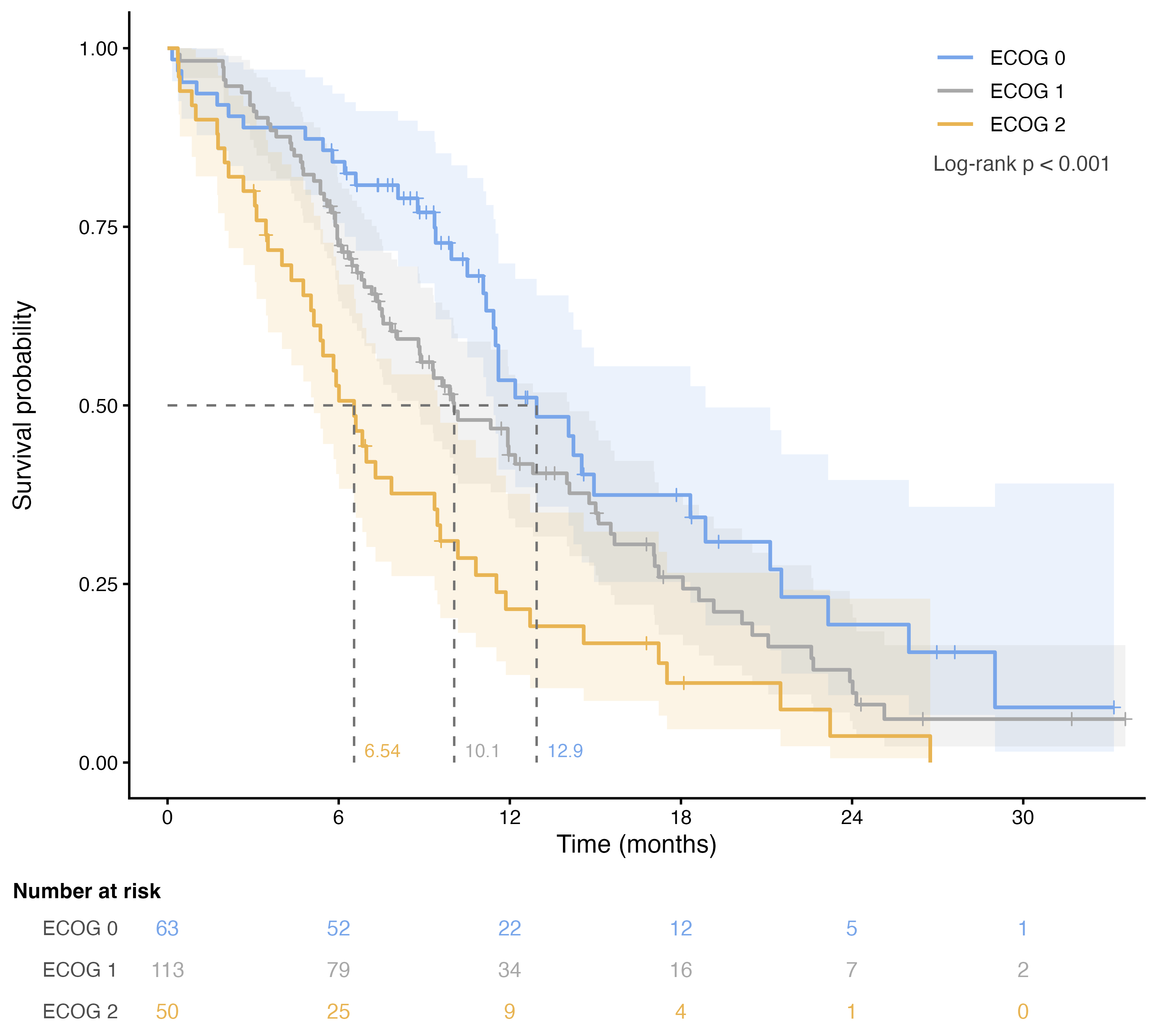
Figure 4: Survival by ECOG as the module draws it, with the options of step 2. The number-at-risk table under the plot is part of the figure: it shows how few patients remain after 24 months.

Read the plot as a sceptical reader would: the curves start at 1 and separate early; the median lines agree with the table; the bands widen to the right as the numbers at risk fall; and after about 24 months the curves rest on a handful of patients.

Step 3: the other views

Tick Cumulative incidence (1 − S), Cumulative hazard and Log-log (PH check) under Plots. They use the same data and the same options.

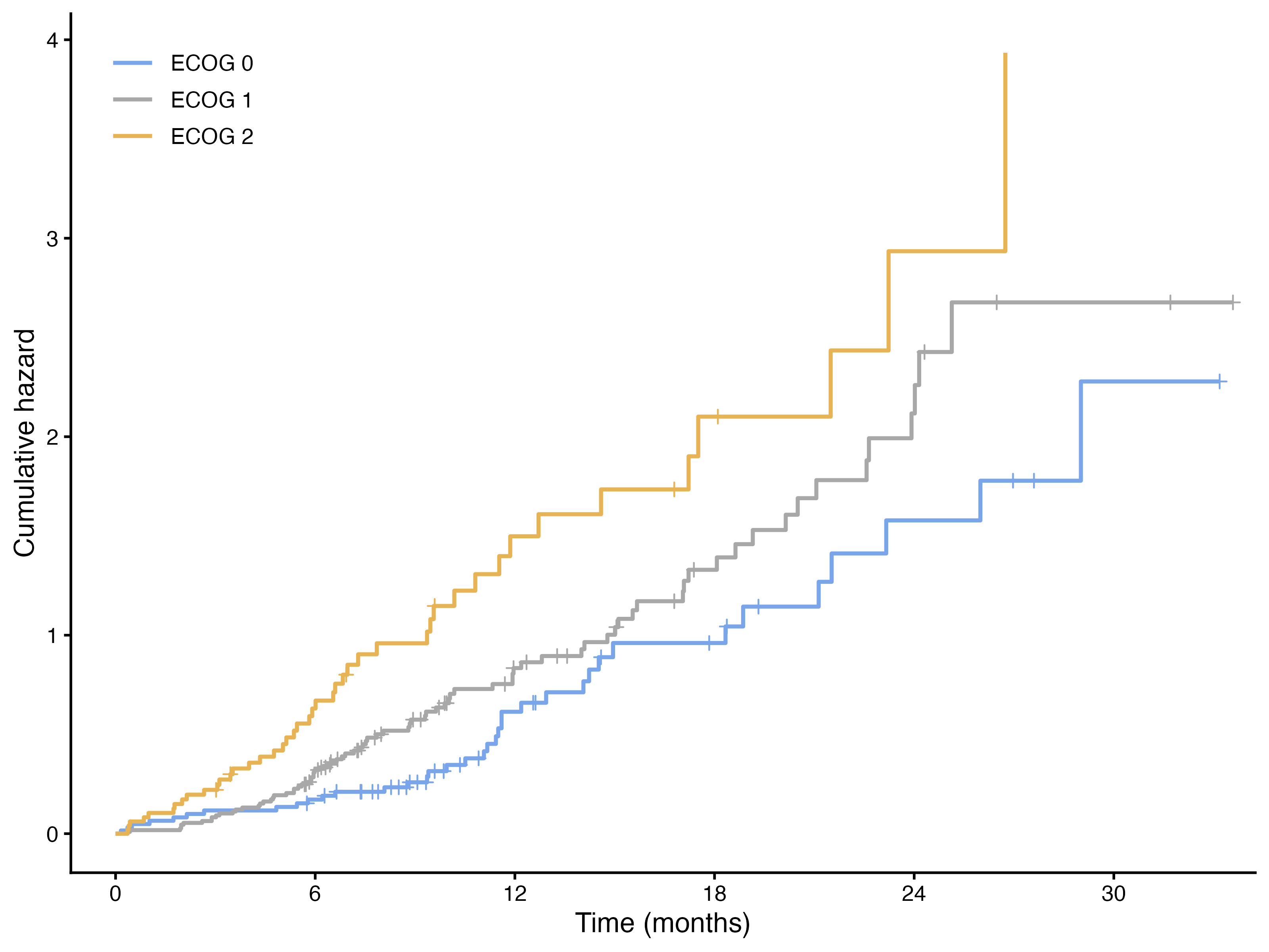
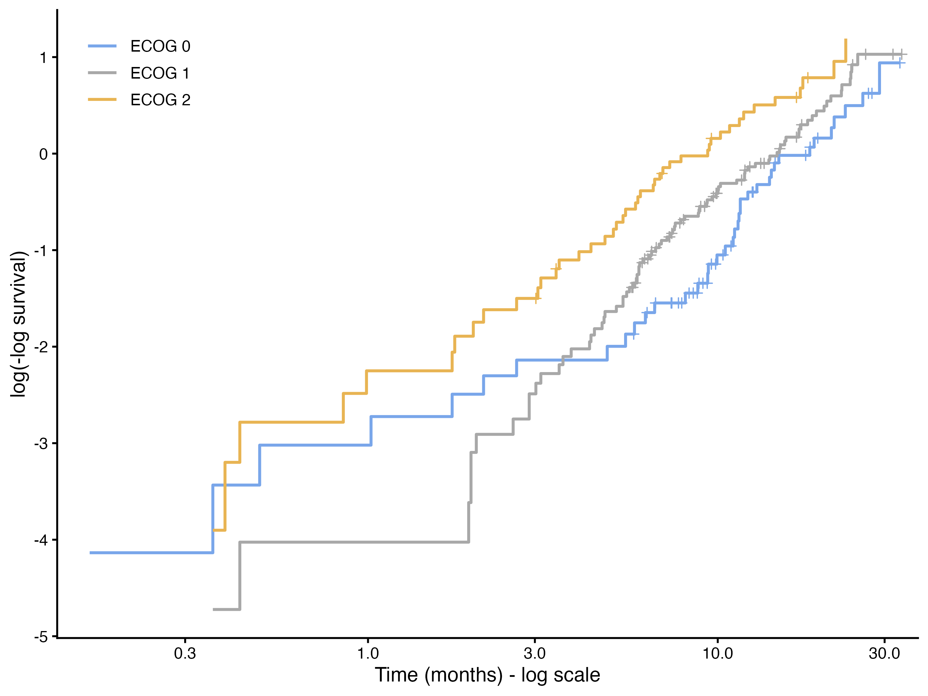
Figure 5: Cumulative hazard by ECOG. The slope of each curve is the hazard: all three get steeper with time (the death rate rises as the disease progresses), and ECOG 2 is the steepest from the start. The last steps on the right rest on very few patients.

Figure 6: The log-log plot: \(\log(-\log \widehat S(t))\) against time on a log scale. Parallel curves support the proportional-hazards assumption of the Cox model; curves that cross or converge are a warning.

ECOG 2 stays above the other two and roughly parallel to them. ECOG 0 and ECOG 1 cross in the first four months, but each step there is a single death, and they come closer again after about a year: a hint, no more, that the difference between ECOG 0 and 1 is not constant over time. The assumptions page checks this formally.

Step 4: write it up

Of 226 patients with advanced non-small-cell lung cancer, 163 died during a median follow-up of 19.3 months (reverse Kaplan-Meier). Median survival was 10.2 months (95% CI 9.4–11.9) and 1-year survival 41% (95% CI 35%–49%). Survival decreased with worse performance status: median 12.9, 10.1 and 6.5 months, and 1-year survival 54%, 43% and 21%, for ECOG 0, 1 and 2 (log-rank χ² = 18.0, 2 df, p < 0.001; test for trend p < 0.001).

What this does not say is whether ECOG predicts survival independently of age and sex. That needs Cox regression.