Interactions: does one effect depend on another?

Testing whether the effect of sex differs by ECOG, hazard ratios within subgroups, a covariate-by-factor interaction, and the subgroup fallacy.

Question. Women had a lower hazard of death than men in the Cox example. Is that advantage the same whatever the performance status, or does it depend on ECOG? This is a question about effect modification (see interactions).

Step 1: add the interaction

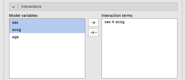
Keep the model of the Cox example (Factors sex, ecog; Covariate age). Open the Interactions section of the panel: the Model variables list holds the factors and covariates of the model. Select sex and ecog together (Ctrl-click, or ⌘-click on a Mac), click the lower arrow, the one with a small menu (→▾), and choose Interaction: the term sex ✻ ecog appears in Interaction terms (Figure 1). The plain arrow above it adds sex and ecog on their own as well; the module ignores those, since they are already in the model.

Figure 1: The Interactions section of the Cox panel with the term sex ✻ ecog.

jamovi syntax

r <- prognosis::cox(data = lung, elapsed = time, event = event, eventLevel = "dead",
                    factors = vars(sex, ecog), covs = age, interactions = ~ sex:ecog,
                    forest = TRUE, showExplanations = TRUE)

Two new tables appear.

Interaction tests

	χ²	df	p
sex × ecog	0.226	2	.893
Note. Likelihood-ratio test for adding the interaction; a small p suggests that the effect of one variable depends on the other.

The interaction test is a likelihood-ratio test comparing the model with and without the interaction terms: χ² = 0.23 on 2 df (one extra coefficient for each combination of a non-reference sex level with a non-reference ECOG level), p = 0.893. There is no evidence that the effect of sex differs between ECOG groups.

Hazard ratios within subgroups

			95% CI
Effect of	Within	HR	Lower	Upper	p
sex: Female – Male	ecog = ECOG 0	0.527	0.247	1.122	.097
	ecog = ECOG 1	0.561	0.353	0.892	.014
	ecog = ECOG 2	0.657	0.349	1.238	.194
Note. Hazard ratio of the first variable within each level (or quartile) of the second; other variables at their reference level or median.

The hazard ratios within subgroups give the effect of the first variable of the term (women versus men) within each level of the second (ECOG). Other variables are held at their reference level or median; since age is not part of the interaction, its value does not change these HRs.

The subgroup fallacy

Only the middle row is “significant” (p = 0.014); the other two are not (p = 0.097 and p = 0.194). It is tempting to conclude that “being a woman is protective only in ECOG 1 patients”. That conclusion is wrong. The three HRs are very similar (0.53, 0.56, 0.66); the ECOG 1 group is simply the largest (113 of 226 patients), so its CI is the narrowest. A significant result in one subgroup and a non-significant one in another is not evidence that the effects differ; the interaction test is, and here it is far from significant (p = 0.893).

Step 2: the coefficient table with an interaction

Hazard ratios

			95% CI
		HR	Lower	Upper	p
sex	Male	1.000
	Female	0.527	0.247	1.12	.097
ecog	ECOG 0	1.000
	ECOG 1	1.489	0.939	2.36	.091
	ECOG 2	2.314	1.366	3.92	.002
age	per unit	1.010	0.991	1.03	.315
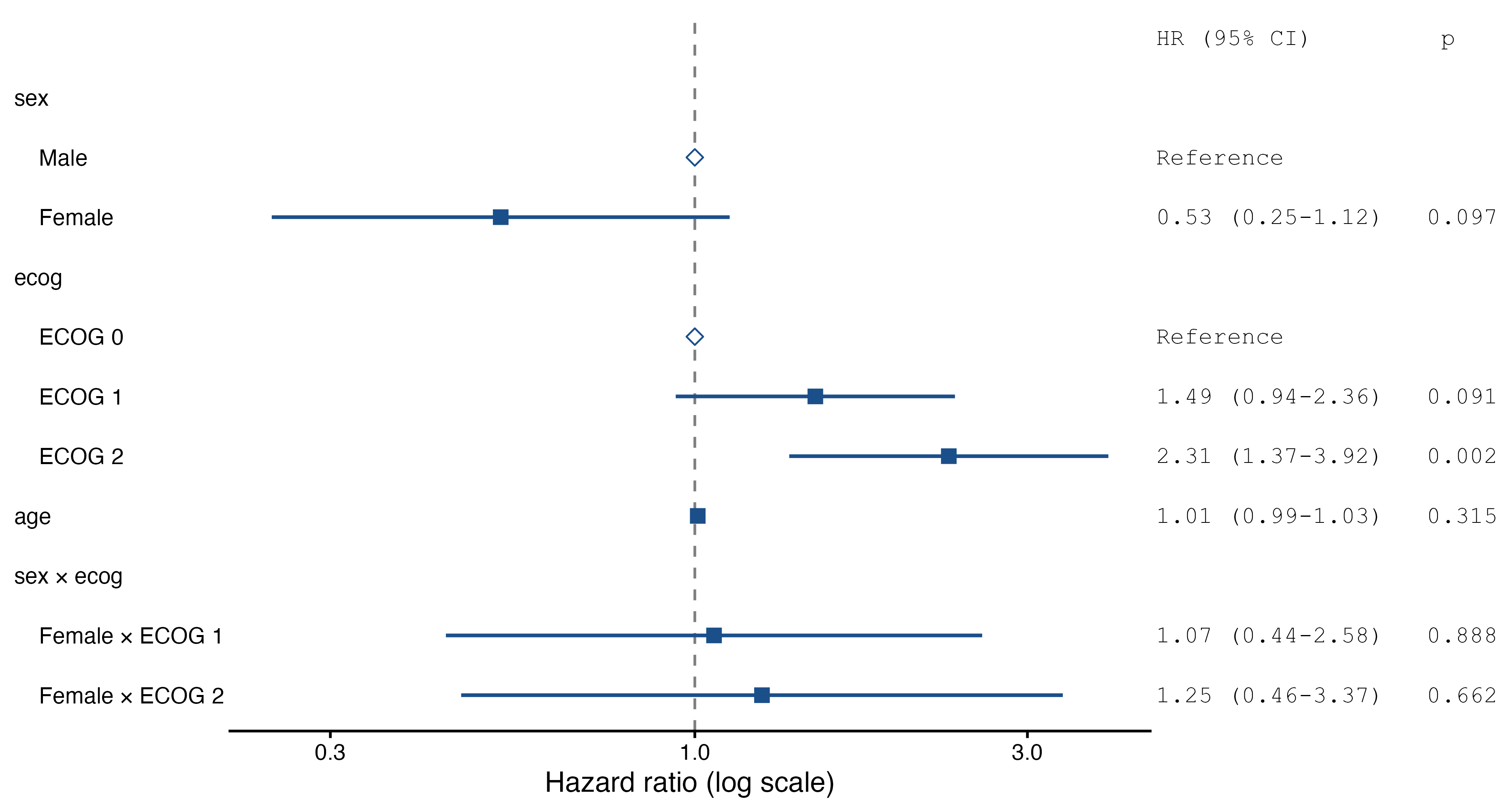
sex × ecog	Female × ECOG 1	1.066	0.439	2.58	.888
	Female × ECOG 2	1.248	0.462	3.37	.662
Note. HR > 1: higher hazard (worse prognosis) than the reference level, or per one-unit increase of a covariate. Multivariable HRs are adjusted for the other variables in the model. With interactions, main-effect HRs apply at the reference level (or 0) of the interacting variable.

With an interaction in the model, the other rows change meaning (the note under the table says so):

Female (HR 0.53) is now the effect of sex in the reference level of ECOG (ECOG 0), which matches the first row of the subgroup table.
ECOG 1 and ECOG 2 are the effects of ECOG in men (the reference level of sex).
The interaction rows (Female × ECOG 1, Female × ECOG 2) are ratios of hazard ratios: how much the female-versus-male HR is multiplied in ECOG 1 or 2 compared with ECOG 0. For example, 0.53 × 1.07 = 0.56, the HR for women in ECOG 1. Values near 1 mean no interaction.

So when you keep an interaction, report the subgroup HRs, not the main-effect rows. When the interaction test is not significant, as here, remove the interaction and report the simpler model of the Cox example.

Figure 2: The forest plot of the model with the interaction: the main effects, then one row for each interaction coefficient.

Step 3: a covariate and a factor

Interactions work the same way with a continuous covariate. Does the effect of age differ between men and women? Replace the interaction by age ✻ sex (select both, choose Interaction again), and set age to per 10 units in Covariate Scaling:

jamovi syntax

ra <- prognosis::cox(data = lung, elapsed = time, event = event, eventLevel = "dead",
                     factors = vars(sex, ecog), covs = age, interactions = ~ age:sex,
                     covScales = list(list(var = "age", scale = "ten")))

Interaction tests

	χ²	df	p
age × sex	1.68	1	.196

Hazard ratios within subgroups

			95% CI
Effect of	Within	HR	Lower	Upper	p
age (per 10 units)	sex = Male	1.214	0.968	1.52	.094
	sex = Female	0.943	0.694	1.28	.705

Each 10 years of age multiplied the hazard by 1.21 in men and by 0.94 in women, but the interaction test is not significant (p = 0.196): the data cannot tell the two effects apart. When one variable is a factor and the other a covariate, the subgroup table always gives the HR of the covariate within each level of the factor, whatever the order of the term. When both are covariates (say age and a laboratory value), it gives the HR of the first at the 25th, 50th and 75th percentiles of the second.

Good practice

Decide on interactions before seeing the data, from a clinical question; every extra interaction tested is another chance of a false positive.
Report the interaction test, not only the subgroup results.
Expect low power. Detecting an interaction as large as the main effect needs about four times the sample size (Brookes et al. 2004). A non-significant interaction test means “no evidence of a difference”, not “the effects are equal”.

References

Brookes, Sara T., Elise Whitely, Matthias Egger, George Davey Smith, Paul A. Mulheran, and Tim J. Peters. 2004. “Subgroup Analyses in Randomized Trials: Risks of Subgroup-Specific Analyses; Power and Sample Size for the Interaction Test.” Journal of Clinical Epidemiology 57 (3): 229–36. https://doi.org/10.1016/j.jclinepi.2003.08.009.