Cox regression in jamovi

Univariable and multivariable hazard ratios for sex, ECOG and age: the model summary, the tests, the HR table, per-10-year HRs and the forest plot.

Question. The Kaplan-Meier example showed that survival falls with worse ECOG. Does ECOG still predict survival once age and sex are taken into account? And are age and sex prognostic themselves?

Step 1: the panel

Open Analyses → Prognosis → Cox Regression and set:

Panel	Setting
Time	`time`
Event	`event`; Event level `dead`
Factors	`sex`, `ecog`
Covariates	`age`
Hazard ratios	Univariable and multivariable; Trend test (p)
Model	Global tests (LR, Wald, score) (on by default)
Options	Show explanations

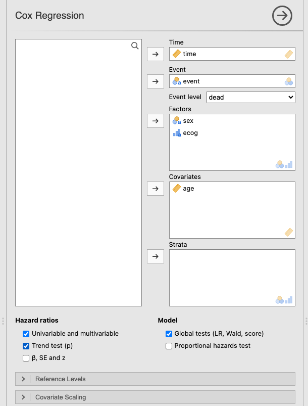
Figure 1: *Prognosis → Cox Regression* in jamovi, set as in the table above (the options panel).

The results appear once the time, the event level and at least one factor or covariate are set. The module uses the patients with no missing value in any model variable; if some are excluded, a note under the model summary says how many. Here all 226 patients are complete. The univariable models are fitted on the same patients as the multivariable one, so the two columns are comparable.

jamovi syntax

r <- prognosis::cox(data = lung, elapsed = time, event = event, eventLevel = "dead",
                    factors = vars(sex, ecog), covs = age, uniMulti = TRUE, trend = TRUE,
                    showExplanations = TRUE)

Step 2: model summary and global tests

Model summary

			95% CI
N	Events	C-index	Lower	Upper
226	163	0.635	0.585	0.684
Note. C-index: probability that, of two patients, the one who has the event first has the higher predicted risk (0.5 = chance, 1 = perfect).

Global tests

	χ²	df	p
Likelihood ratio	28.9	4	< .001
Wald	28.6	4	< .001
Score (log-rank)	29.7	4	< .001
Note. H0: all hazard ratios in the model are 1.

163 deaths among 226 patients support the four coefficients of this model comfortably (about 41 events per coefficient).

The C-index is 0.635: for two patients whose order of death is known, the model gives the higher risk to the one who died first 63% of the time (chance would be 50%). That is modest, and typical for a few clinical variables.

The three global tests agree (likelihood ratio χ² = 28.9 on 4 df, p < 0.001): at least one of the variables is associated with survival. Report one of them, usually the likelihood-ratio test.

Step 3: the hazard ratio table

Hazard ratios

		Univariable					Multivariable
		HR	Lower	Upper	p	p trend	HR	Lower	Upper	p	p trend
sex	Male	1.000			.002	.002	1.000				.001
	Female	0.596	0.429	0.828	.002		0.579	0.417	0.806	.001
ecog	ECOG 0	1.000			< .001	< .001	1.000				< .001
	ECOG 1	1.446	0.979	2.134	.064		1.507	1.019	2.228	.040
	ECOG 2	2.498	1.608	3.878	< .001		2.465	1.577	3.855	< .001
age	per unit	1.019	1.000	1.037	.046		1.011	0.993	1.029	.247
Note. HR > 1: higher hazard (worse prognosis) than the reference level, or per one-unit increase of a covariate. Multivariable HRs are adjusted for the other variables in the model. Univariable: each variable alone; on the reference row, p of the Wald test for the whole variable. p trend: the factor entered as a numeric score (level order); multivariable trend keeps the other variables as in the model.

How to read it:

Reference rows. Male and ECOG 0 are the reference levels (the first level of each factor): HR = 1 by definition, no CI. In the univariable columns, the p on the reference row is the Wald test of the whole variable (for ECOG, 2 df: do the three levels differ?), and p trend is the 1-df test of a steady change along the levels.
ECOG. Adjusted for sex and age, ECOG 1 patients had 1.51 times the hazard of death of ECOG 0 patients (95% CI 1.02–2.23), and ECOG 2 patients 2.47 times (1.58–3.86). The trend test, p < 0.001, summarises it: the hazard rises with each step of ECOG. Note that ECOG 1 versus 0 is not significant in the univariable column (p = 0.064) but is after adjustment (p = 0.040); the estimates themselves barely move (1.45 and 1.51).
Sex. Women had a lower hazard than men: HR 0.58 (0.42–0.81) adjusted, 0.60 crude. Adjustment changes almost nothing: sex is not confounded by age or ECOG here.
Age. This is the interesting row. Alone, each year of age multiplied the hazard by 1.019 (1.000–1.037, p = 0.046). Adjusted for sex and ECOG, the HR shrinks to 1.011 (0.993–1.029, p = 0.247). Part of the crude age effect was confounding by ECOG: older patients more often had a poor performance status (mean age 66 years with ECOG 2 versus 61 with ECOG 0–1), and it is the performance status that carries most of the prognostic information.

Changing the reference level

The first level of a factor is its reference. To compare against another level (for example to report men versus women), open the variable’s Setup in the Data tab and move that level to the top. The HR becomes its reciprocal, 1/0.58 = 1.73, the CI limits are inverted in the same way, and the p-values do not change.

Step 4: hazard ratios per 10 years

“1.019 per year” is correct but hard to grasp. Open Covariate Scaling, which lists every covariate, and set age to per 10 units:

jamovi syntax

r10 <- prognosis::cox(data = lung, elapsed = time, event = event, eventLevel = "dead",
                      factors = vars(sex, ecog), covs = age, uniMulti = TRUE,
                      covScales = list(list(var = "age", scale = "ten")), coefDetails = TRUE)

Hazard ratios

		Univariable				Multivariable
		HR	Lower	Upper	p	HR	Lower	Upper	p	β	SE	z
sex	Male	1.000			.002	1.000
	Female	0.596	0.429	0.828	.002	0.579	0.417	0.806	.001	-0.546	0.1682	-3.24
ecog	ECOG 0	1.000			< .001	1.000
	ECOG 1	1.446	0.979	2.134	.064	1.507	1.019	2.228	.040	0.410	0.1996	2.05
	ECOG 2	2.498	1.608	3.878	< .001	2.465	1.577	3.855	< .001	0.902	0.2281	3.96
age	per 10 units	1.203	1.004	1.442	.046	1.114	0.928	1.337	.247	0.108	0.0931	1.16

The age row now reads per 10 units: the crude HR is 1.20 per 10 years of age (1.203 = 1.019¹⁰), the adjusted one 1.11. The module divides age by 10 before fitting, so only the unit changes: the p-values, the other HRs and the model tests are the same as before. Per 1 SD does the same with the standard deviation of the variable, which helps to compare continuous variables measured in different units.

This run also ticked β, SE and z, the columns behind each HR: \(\mathrm{HR} = e^{\beta}\), its 95% CI is \(e^{\beta \pm 1.96\,\mathrm{SE}}\), and \(z = \beta/\mathrm{SE}\) gives the p-value. For ECOG 2, \(e^{0.902} = 2.47\) and \(e^{0.902 \pm 1.96 \times 0.228}\) gives 1.58–3.86.

Step 5: the forest plot

Tick Forest plot under Plots. With Univariable and multivariable on, it shows both estimates for each row:

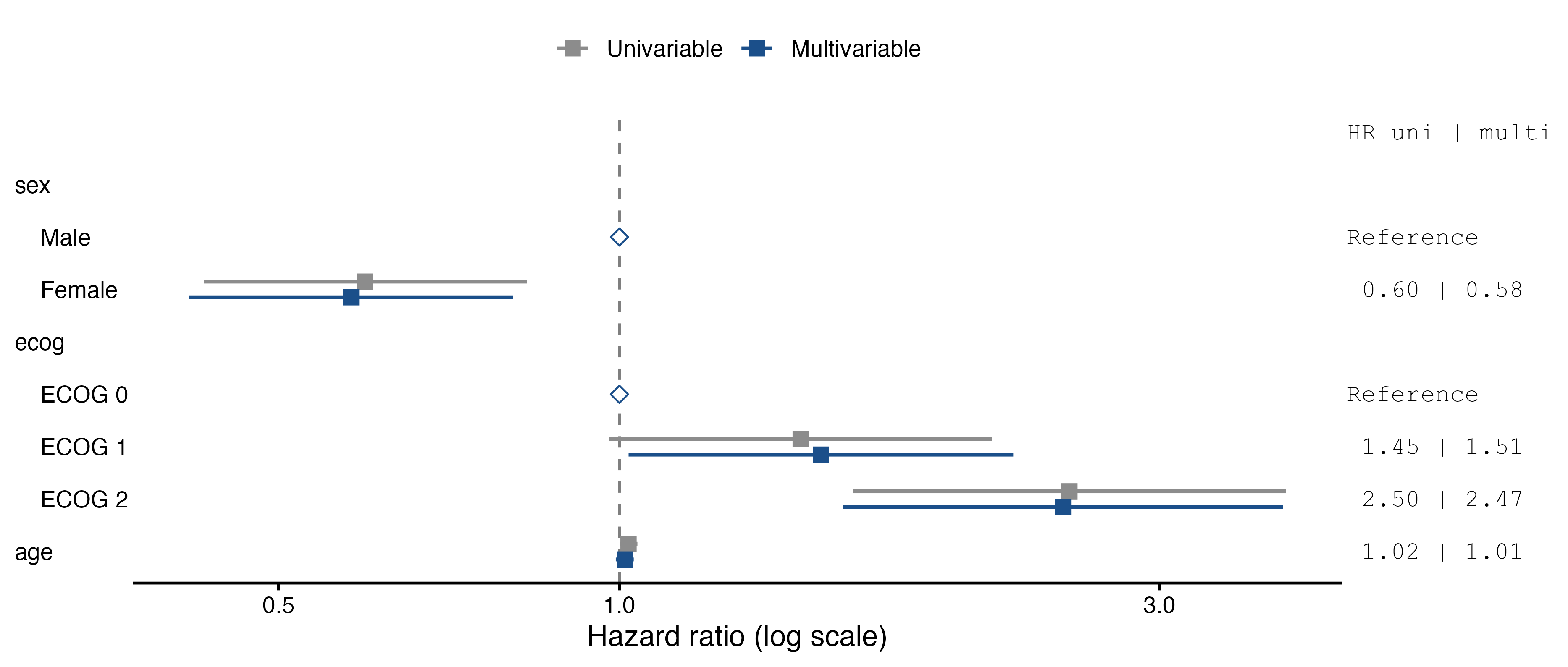
Figure 2: Forest plot of the hazard ratios, univariable (grey) and multivariable (blue), on a log scale. Diamonds mark the reference levels. The dashed line is HR = 1.

The log scale makes HR = 0.5 and HR = 2 equally far from 1, as they should be: halving and doubling the hazard are effects of the same size.

Step 6: write it up

In a Cox model including sex, age and ECOG performance status (226 patients, 163 deaths), survival was worse with higher ECOG: HR 1.51 (95% CI 1.02–2.23) for ECOG 1 and 2.47 (95% CI 1.58–3.86) for ECOG 2, compared with ECOG 0 (p for trend < 0.001). Women had a lower hazard of death than men, HR 0.58 (95% CI 0.42–0.81). Age was associated with survival in the univariable analysis, HR per 10 years 1.20 (95% CI 1.00–1.44), but not after adjustment, 1.11 (95% CI 0.93–1.34). The model C-index was 0.63.

Before trusting these numbers, check the proportional-hazards assumption: Assumptions.