Adjusted survival curves

Survival curves by ECOG adjusted for sex and age by direct standardisation, compared with the unadjusted Kaplan-Meier curves.

Question. The Kaplan-Meier curves by ECOG compare groups that also differ in age and in the proportion of women. What would the curves look like if the three ECOG groups had the same age and sex distribution?

Hazard ratios answer this on the hazard scale; adjusted survival curves answer it on the scale of survival probabilities, which is easier to communicate.

Step 1: the panel

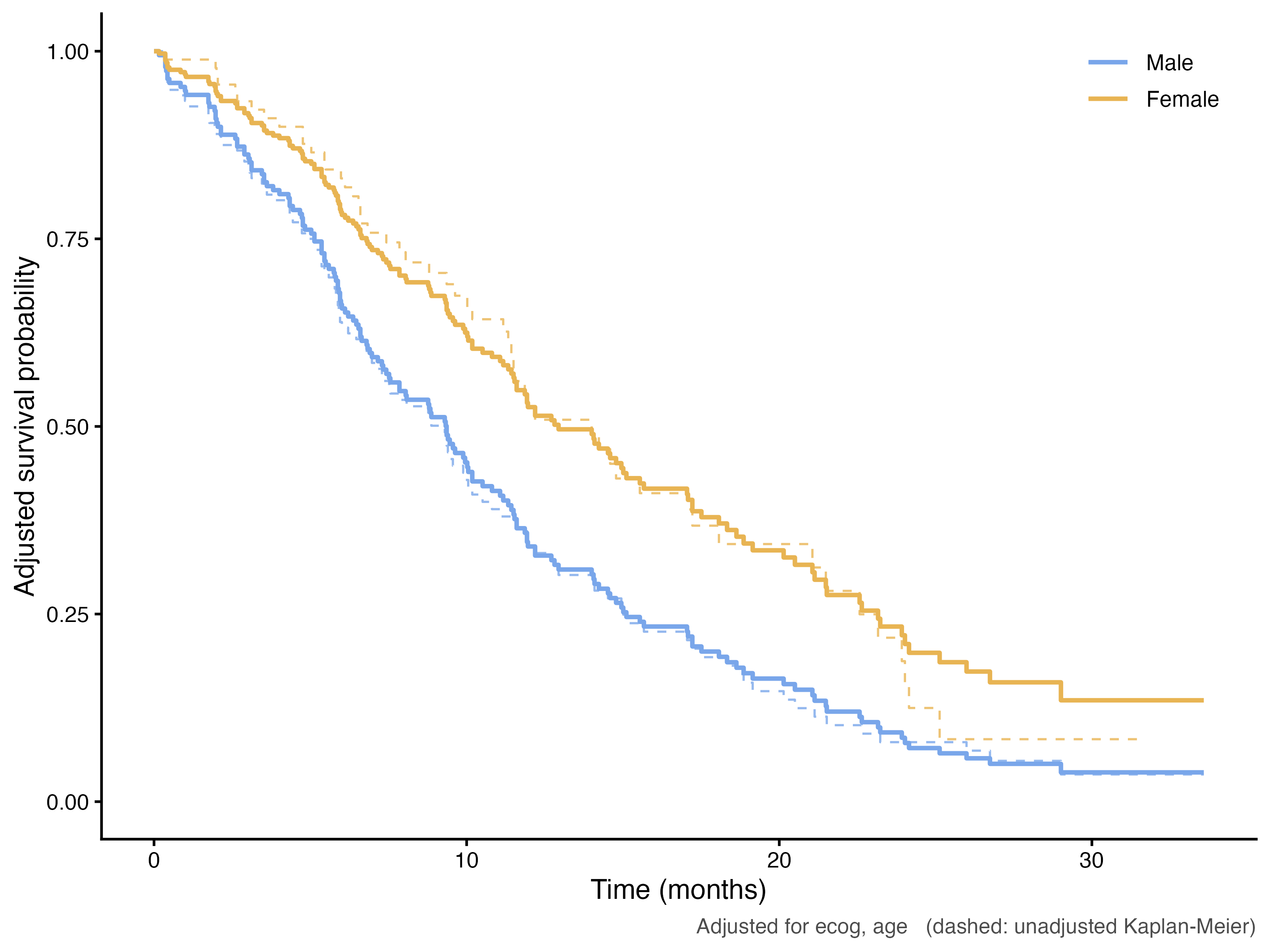
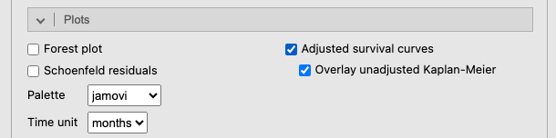
In the Cox model of the Cox example (Factors sex, ecog; Covariate age), tick Adjusted survival curves under Plots (Figure 1). Overlay unadjusted Kaplan-Meier is on by default; Time unit labels the time axis.

Figure 1: The Plots section of the Cox panel with adjusted curves ticked.

jamovi syntax

r <- prognosis::cox(data = lung, elapsed = time, event = event, eventLevel = "dead",
                    factors = vars(sex, ecog), covs = age, adjCurves = TRUE,
                    timeUnit = "months")

The module draws one plot for each factor of the model; covariates such as age get no plot.

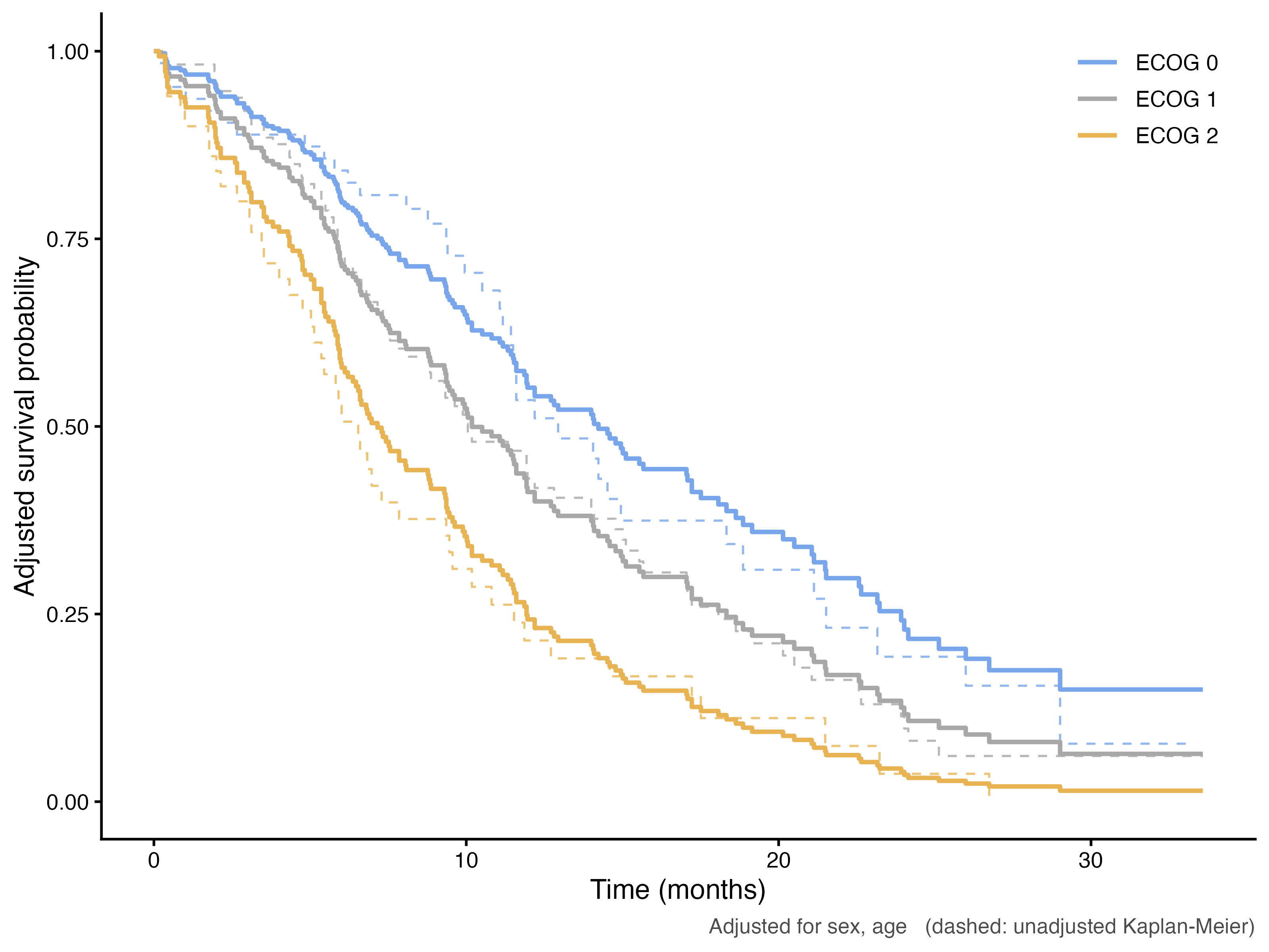
Figure 2: Survival by ECOG adjusted for sex and age (solid), with the Kaplan-Meier curves of the same groups (dashed). The caption under the plot lists the variables adjusted for.

How the curves are computed

The module uses direct standardisation (Makuch 1982). For the ECOG 0 curve, it takes every patient in the data, sets their ECOG to 0 while keeping their own sex and age, predicts their survival curve from the Cox model, and averages the 226 curves:

\[\widehat S_{\text{ECOG }0}(t) = \frac{1}{n}\sum_{i=1}^{n} \widehat S\bigl(t \mid \text{ECOG } 0,\ \text{sex}_i,\ \text{age}_i\bigr)\]

and the same for ECOG 1 and ECOG 2. The three curves describe the same population (the whole cohort) under three performance statuses, so their differences are due to ECOG alone, as far as the model is right. They are not the curves of the patients who actually had each ECOG; the Kaplan-Meier curves are.

Step 2: compare with the unadjusted curves

Survival at 12 months, read from the curves of the plot.
ECOG	Kaplan-Meier	Adjusted for sex and age
ECOG 0	54%	55%
ECOG 1	43%	41%
ECOG 2	21%	24%

The adjusted and unadjusted curves are close. The ECOG 2 group was older than the others, and adjusting for age moves its curve up only slightly: as the Cox example showed, once ECOG is known age adds little. The difference between the ECOG groups is not explained by age or sex.

When the dashed and solid curves are far apart, the groups differed in the adjustment variables, and the Kaplan-Meier comparison was confounded.

Figure 3: The same for sex, adjusted for ECOG and age.

Limits

The curves are only as good as the Cox model: they assume proportional hazards and the log-linear effect of age.
They are not available for stratified models; the module shows a message instead.
Adjusted curves are an average over the patients in the data: with a different case mix, the curves would be different, even with the same hazard ratios.

References

Makuch, Robert W. 1982. “Adjusted Survival Curve Estimation Using Covariates.” Journal of Chronic Diseases 35 (6): 437–43. https://doi.org/10.1016/0021-9681(82)90058-3.