jamovi syntax
r <- prognosis::cox(data = lung, elapsed = time, event = event, eventLevel = "dead",
                    factors = vars(sex, ecog), covs = age, ph = TRUE, phPlot = TRUE,
timeUnit = "months", showExplanations = TRUE)The Cox model of the previous example reports one hazard ratio per variable, valid at every time of follow-up. That is an assumption, and it has to be checked (see proportional hazards).
In the same Cox analysis, tick Proportional hazards test (under Model) and Schoenfeld residuals (under Plots):
r <- prognosis::cox(data = lung, elapsed = time, event = event, eventLevel = "dead",
factors = vars(sex, ecog), covs = age, ph = TRUE, phPlot = TRUE,
timeUnit = "months", showExplanations = TRUE)Proportional hazards test
| χ² | df | p | |
|---|---|---|---|
| sex | 2.440 | 1 | .118 |
| ecog | 2.871 | 2 | .238 |
| age | 0.163 | 1 | .686 |
| Global | 4.992 | 4 | .288 |
| Note. Test based on Schoenfeld residuals; a small p suggests that the hazard ratio changes over time (non-proportional hazards). | |||
There is one row per variable (ECOG, with two coefficients, is tested on 2 df) and a global test for the whole model. A small p-value would suggest that the HR of that variable changes over time. Here none is small: p = 0.12 for sex, 0.24 for ECOG and 0.69 for age, and 0.29 globally. There is no evidence against proportional hazards, but “no evidence” is not proof: with 163 deaths the test can miss a moderate change. Look at the plot too.
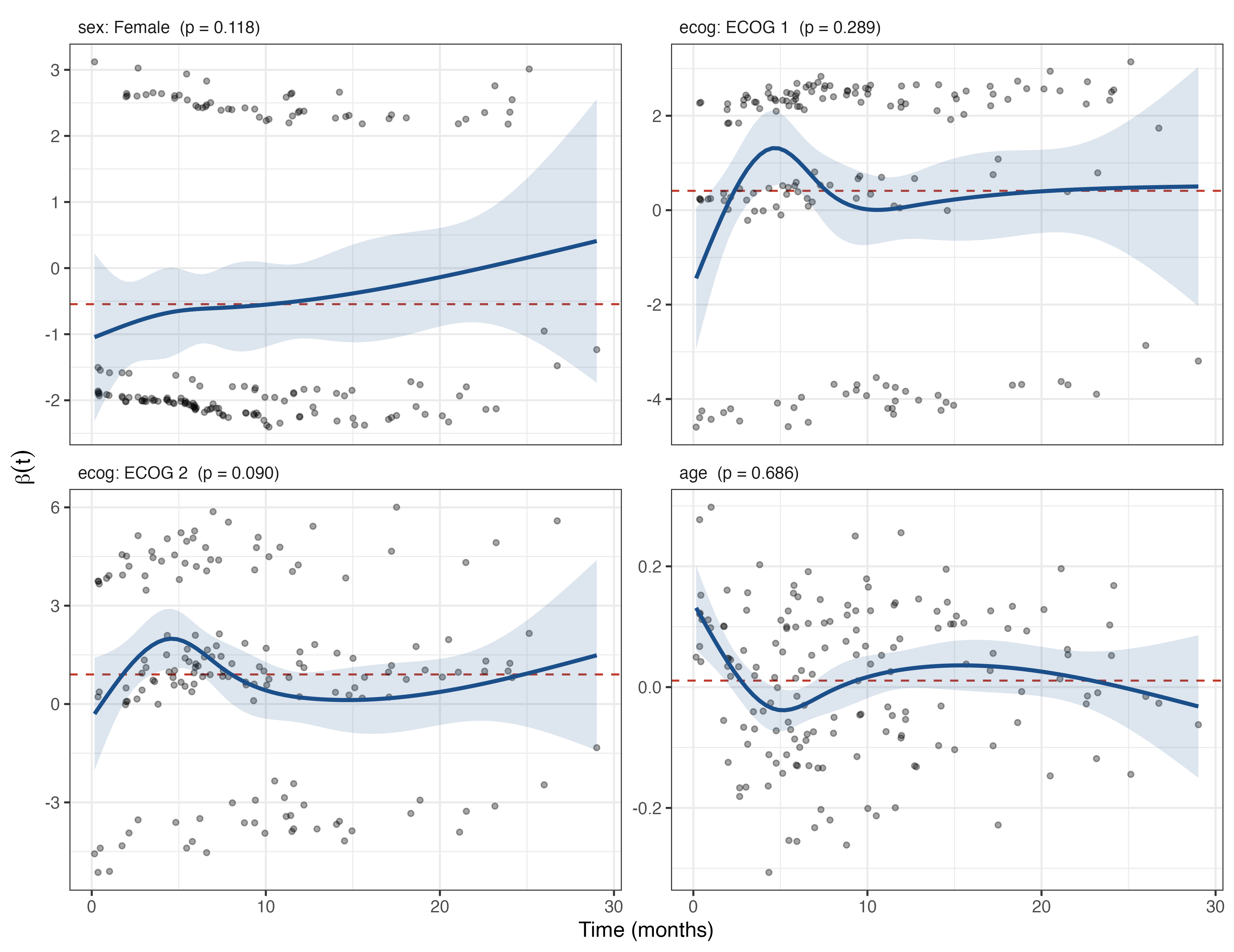
How to read it:
Here the plot shows something the table does not. In roughly the first six months, the curves for both ECOG coefficients rise above the dashed line, and their bands briefly exclude it: the effect of ECOG looks stronger early. This fits the log-log plot of the Kaplan-Meier example, where the ECOG 1 curve starts below ECOG 0 (the very first deaths happened to be in ECOG 0) and overtakes it within a few months. Age shows a similar early wiggle. After that, the curves settle around the dashed lines. For sex the curve drifts upward (towards less protection) late in follow-up, where there are few deaths and the band is wide.
Why do the test and the plot seem to disagree? The test looks for a steady trend of β(t) over the whole follow-up, and a bump in the first months followed by a flat stretch is not a trend. The band is pointwise: over many time points, it will exclude the line somewhere by chance fairly often. The fair reading is: there is no strong evidence against proportional hazards, the single HR for ECOG is a reasonable summary, and there are hints that its effect is largest in the first half-year. A paper about ECOG itself could report that, for example with survival at 6 and 12 months or separate HRs for early and late follow-up (step 3).
The log-log plot of the Kaplan-Meier analysis is the graphical check for one factor at a time without adjustment; the residuals check each coefficient of the adjusted model, including continuous covariates such as age, which the log-log plot cannot handle.
When a variable clearly violates proportional hazards, there are honest options:
What not to do: drop the variable because its test was significant, or switch to another test because its p-value is smaller.
Suppose sex had failed the test. Move sex from Factors to Strata:
rs <- prognosis::cox(data = lung, elapsed = time, event = event, eventLevel = "dead",
                     factors = ecog, covs = age, strata = sex, ph = TRUE)
Model summary
| 95% CI | ||||
|---|---|---|---|---|
| N | Events | C-index | Lower | Upper |
| 226 | 163 | 0.604 | 0.552 | 0.656 |
| Note. Stratified by sex | ||||
Hazard ratios
| 95% CI | |||||
|---|---|---|---|---|---|
| HR | Lower | Upper | p | ||
| ecog | ECOG 0 | 1.00 | |||
| ECOG 1 | 1.44 | 0.972 | 2.14 | .069 | |
| ECOG 2 | 2.46 | 1.570 | 3.84 | < .001 | |
| age | per unit | 1.01 | 0.992 | 1.03 | .277 |
Men and women now have separate baseline hazards of any shape, and sex has no HR any more. The ECOG hazard ratios (1.44 and 2.46) are close to those of the unstratified model (1.51 and 2.47), as expected when sex’s effect was in fact roughly proportional. The C-index is lower (0.604) because it now only compares patients of the same sex: the part of the prediction that came from sex is gone.
A stratified model cannot give adjusted survival curves: with a separate baseline per stratum, there is no single curve to adjust.