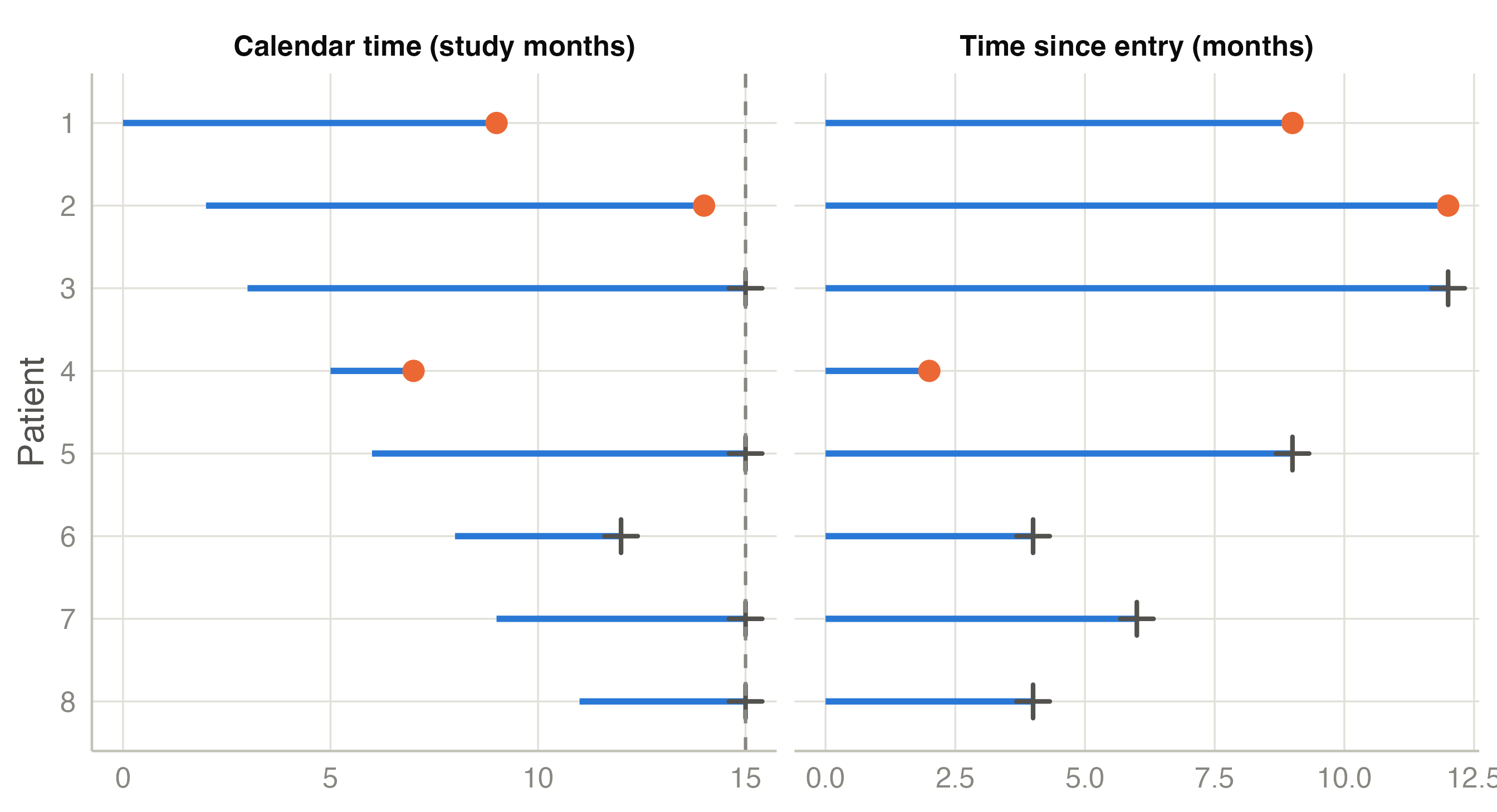
Every time-to-event analysis starts by fixing three things, and a paper that does not state them clearly cannot be interpreted:
For each patient we then observe a pair \((t_i, \delta_i)\): the time \(t_i\) from the origin to the end of observation, and an indicator \(\delta_i\) that says whether observation ended because the event happened (\(\delta_i = 1\)) or for some other reason (\(\delta_i = 0\)). In the teaching dataset these are the columns time (months) and event (dead or alive).
A patient whose observation ends before the event is censored. Their survival time is not missing: we know it is longer than \(t_i\). This is called right censoring, because the true time lies somewhere to the right of what we saw. It happens for ordinary reasons:
The key assumption of every method in this tutorial is non-informative censoring: patients who are censored at a given time must have the same prospects as those who remain under observation. Administrative censoring is usually harmless. Loss to follow-up may not be: if the sickest patients stop coming to the clinic, the patients who remain look healthier than the cohort really is, and survival is overestimated. No statistical method can repair this. Keep loss to follow-up low and report how much there was.
Suppose you want the typical survival of the 226 patients. Some obvious shortcuts all give the wrong answer:
| Approach | Median (months) |
|---|---|
| Median of all observed times (censored treated as deaths) | 8.6 |
| Median time of the patients who died (censored dropped) | 7.5 |
| Kaplan-Meier median (next page) | 10.2 |
Treating a censored time as if the patient had died underestimates survival: the patient lived longer. Dropping censored patients also underestimates it, because the patients still alive at the end of the study are often the long survivors. And the proportion who died, 163/226 = 72%, is not a probability of anything: it depends on how long each patient happened to be followed. A t-test or a linear regression of time has the same problems. Logistic regression of “dead at 12 months” works only for patients followed for at least 12 months and ignores when the deaths happened.
Survival methods use each patient for exactly as long as they were observed, and no longer.
\[S(t) = P(T > t)\]
is the probability of being event-free beyond time \(t\). It starts at \(S(0) = 1\) and can only go down. “Two-year survival is 12 %” is a statement about \(S(24 \text{ months})\). The median survival is the time at which \(S(t)\) falls to 0.5. The Kaplan-Meier curve is an estimate of \(S(t)\).
The hazard is the rate at which events happen at time \(t\) among the patients who are still event-free just before \(t\):
\[h(t) = \lim_{\Delta t \to 0} \frac{P(t \le T < t + \Delta t \mid T \ge t)}{\Delta t}\]
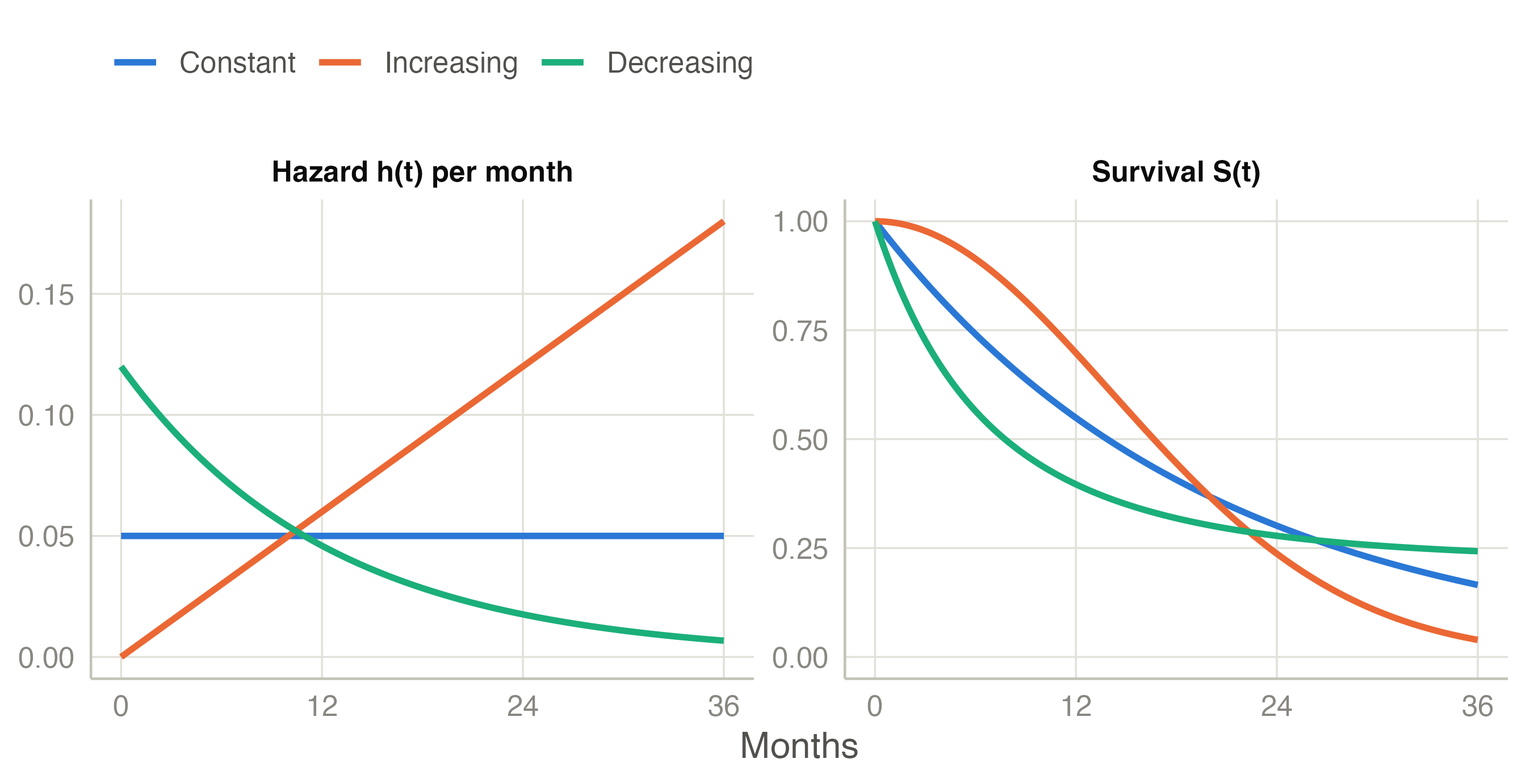
Think of it as the death rate of the patients still alive at that moment, for example “3% per month at month 6”. The hazard can rise, fall or stay constant over time, and its shape tells a clinical story (Figure 2): the risk after surgery is highest in the first days, the risk of death with age increases, and the risk of a chronic disease may be constant.
A hazard is a rate, not a probability, so it has a unit (per month, per year) and can be larger than 1. The ratio of two hazards, the hazard ratio (HR), has no unit; it is what Cox regression estimates.
\[H(t) = \int_0^t h(u)\,du, \qquad S(t) = e^{-H(t)}\]
adds the hazard up over time. With a constant hazard \(h\), \(H(t) = h\,t\). \(H(t)\) can be read roughly as the expected number of events a patient would have had by time \(t\) if the event could repeat.