Teaching with studysim

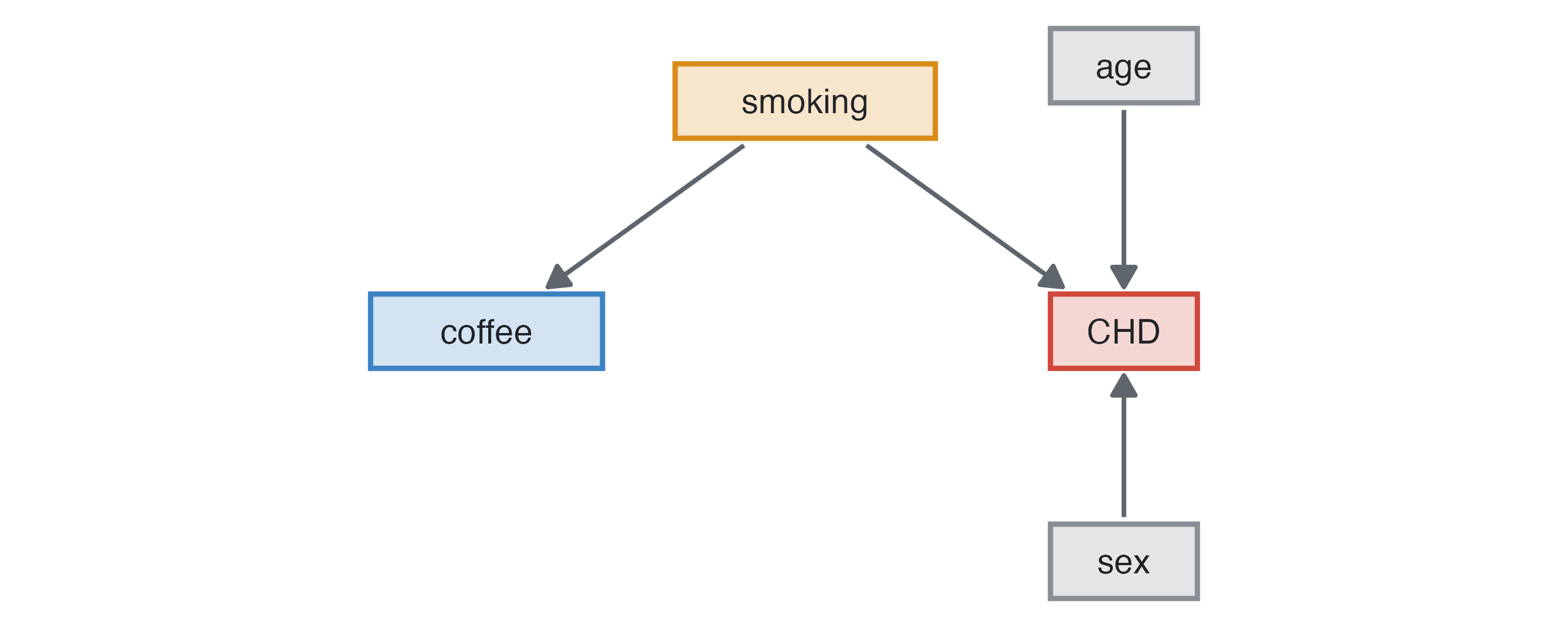
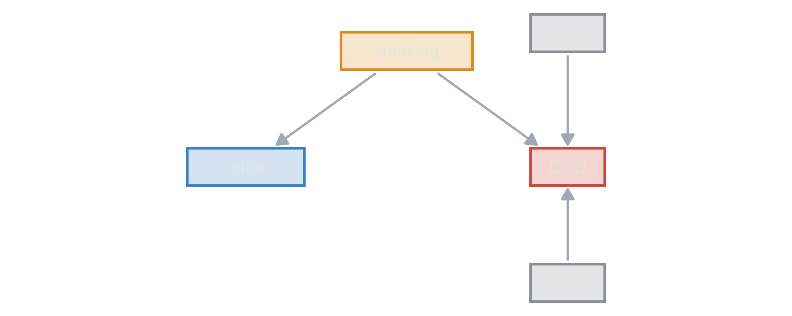
Each exercise below names the scenario and options, then what the students should find. The tables are the answer key’s expected estimates (the average of large simulated studies), computed by the module itself when this page was built. True is the direct effect the data were generated with (every other variable fixed); where a variable also acts through others, the total effect follows, and Adjusted (DAG) adjusts each variable only for what it does not cause.

Confounding: coffee and coronary heart disease

Coronary heart disease incidence, cohort, measure age, sex, smoking and coffee. Coffee has no effect, but coffee drinkers smoke more: the crude hazard ratio of coffee is above 1 and disappears once smoking is in the model.

Figure 1: Coffee has no arrow into coronary heart disease, but smoking causes both: the backdoor path coffee ← smoking → CHD makes coffee look harmful until smoking is adjusted for.

Variable	Contrast	True	direct	total	Crude	Adjusted (all)	Adjusted (DAG)	Estimate
age	per 1 years	HR	1.05	1.07	1.07	1.07	1.07	HR
sex	male vs female	HR	1.60	1.76	1.77	1.79	1.79	HR
smoking	former vs never	HR	1.20	1.21	1.21	1.20	1.21	HR
smoking	current vs never	HR	1.60	1.81	1.76	1.75	1.78	HR
coffee	per 1 cups/day	HR	1.00	1.00	1.08	1.01	1.01	HR

Exercise: leave smoking unmeasured and show that the adjusted coffee effect stays biased (residual confounding).

Confounding by indication: chemotherapy

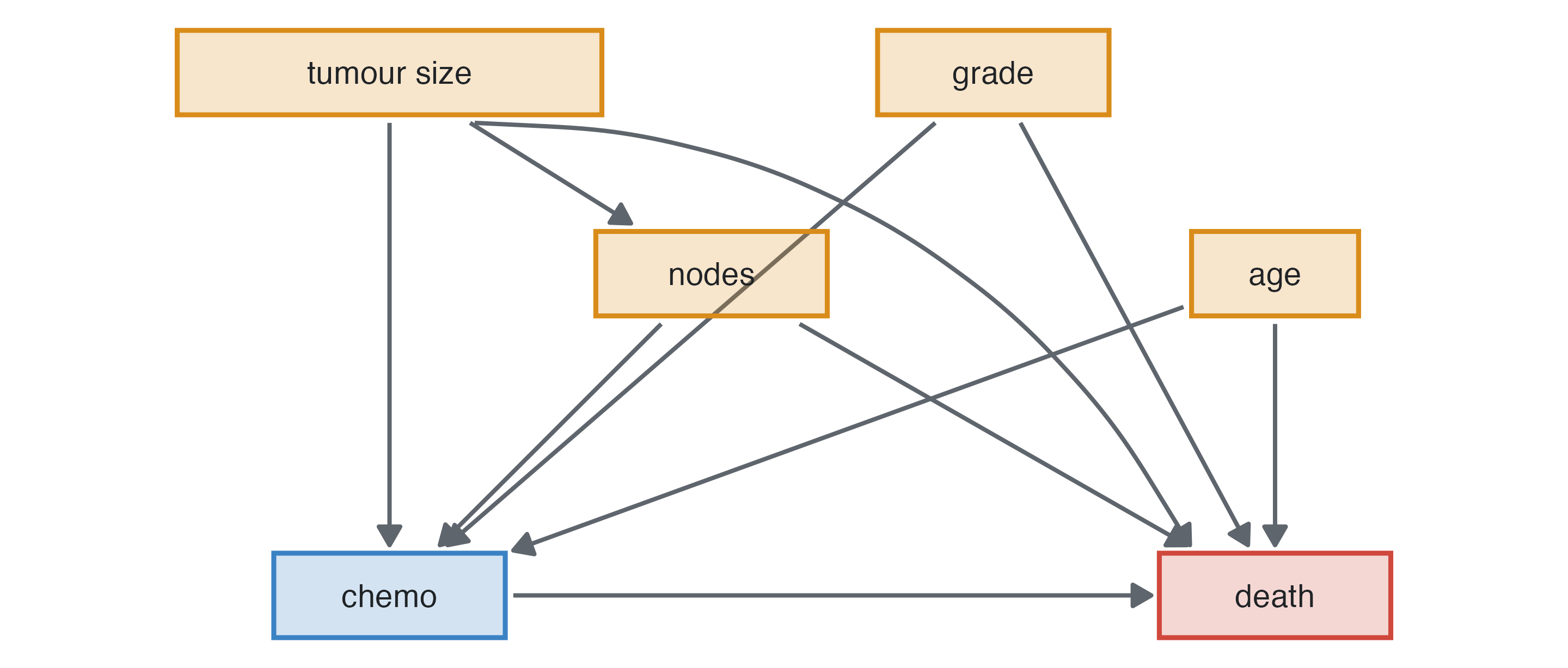
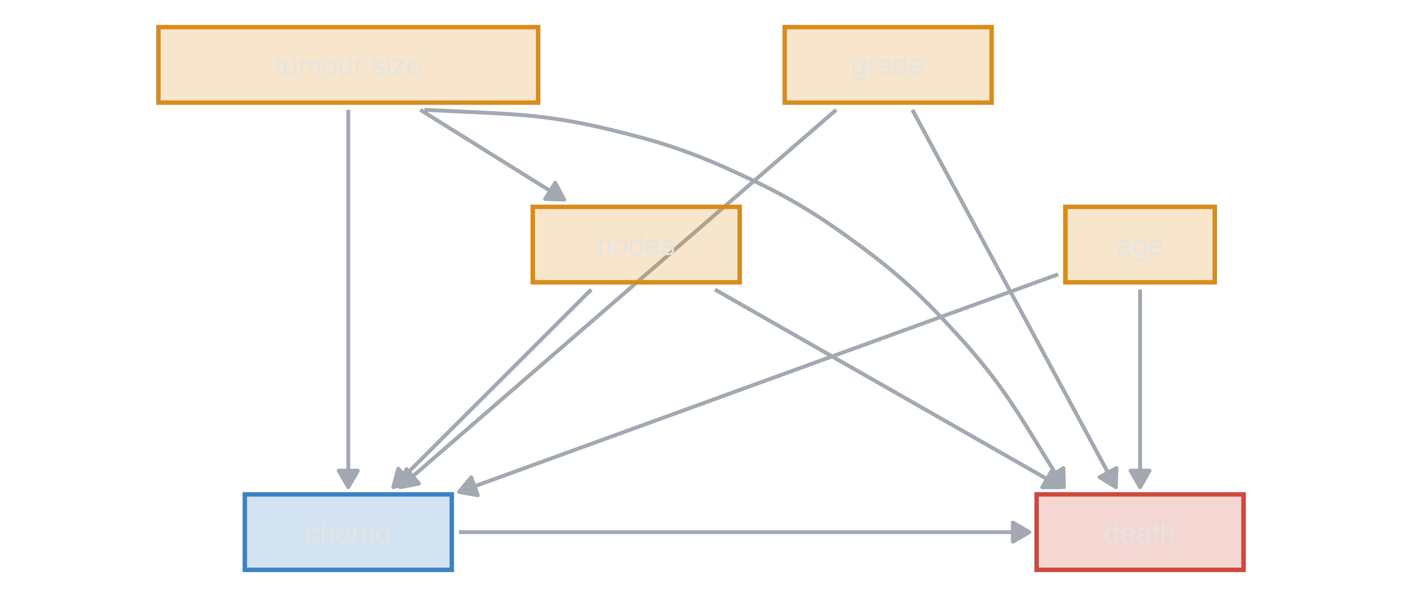
Breast cancer prognosis, prognosis design. Chemotherapy truly lowers the hazard (HR 0.75), but it is given to younger women with more nodes and higher grade; its crude hazard ratio points the wrong way.

Figure 2: Confounding by indication: the worse the tumour (size, nodes, grade) the more likely chemotherapy, and the worse the prognosis. Without adjustment the treatment carries the prognosis of the patients who receive it.

Variable	Contrast	True	direct	total	Crude	Adjusted (all)	Adjusted (DAG)	Estimate
age	per 1 years	HR	1.03	1.03	1.03	1.03	1.03	HR
tumour_size	per 10 mm	HR	1.15	1.19	1.16	1.14	1.16	HR
nodes	per 1	HR	1.08	1.06	1.08	1.08	1.06	HR
grade	G2 vs G1	HR	1.50	1.68	1.56	1.64	1.56	HR
grade	G3 vs G1	HR	2.20	2.75	2.48	2.77	2.50	HR
chemo	yes vs no	HR	0.75	0.75	1.09	0.76	0.76	HR

Odds ratios from a case-control study

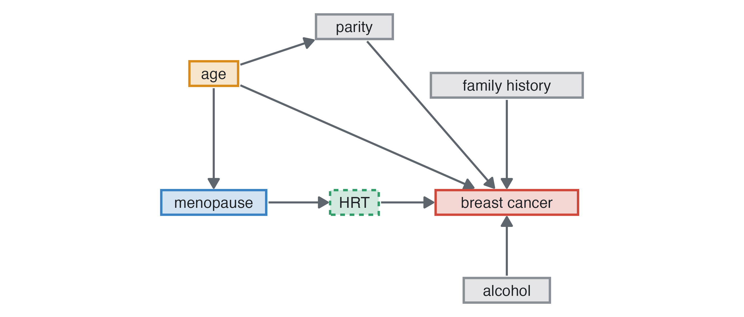
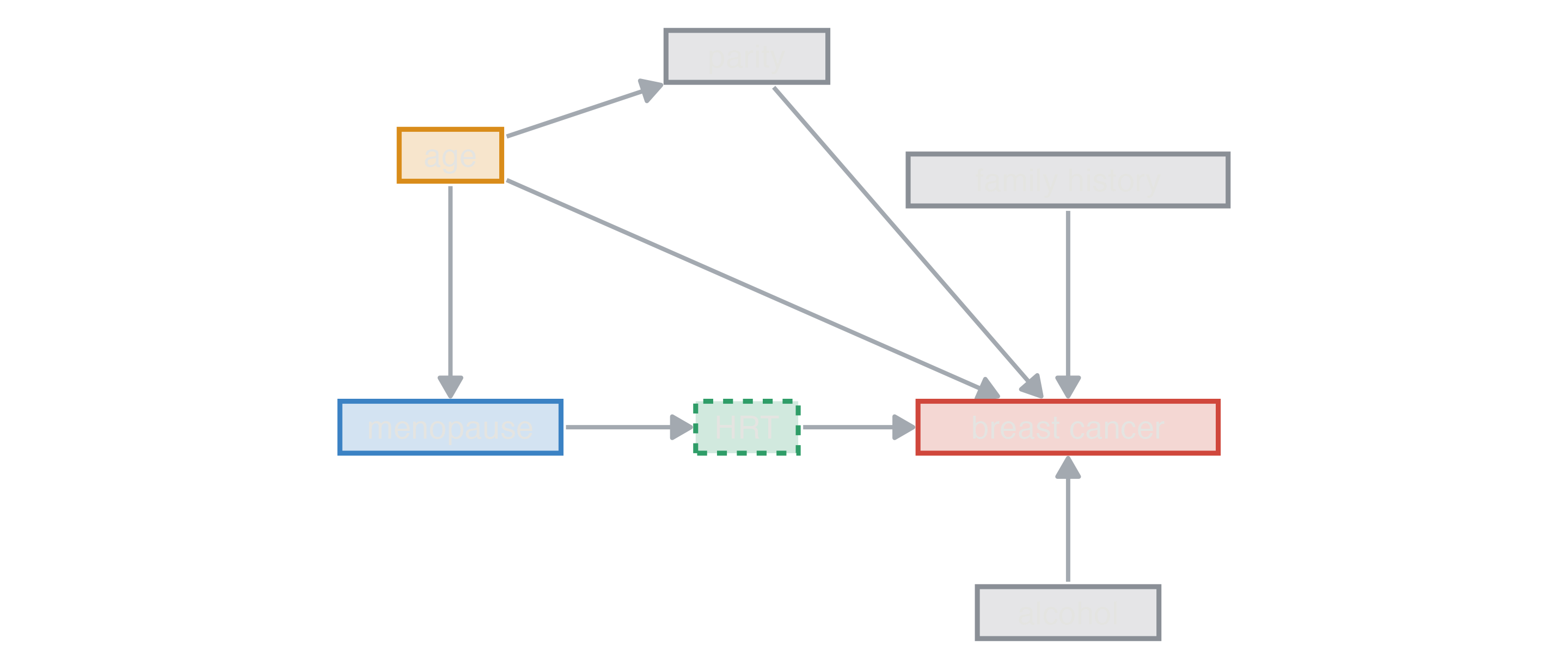
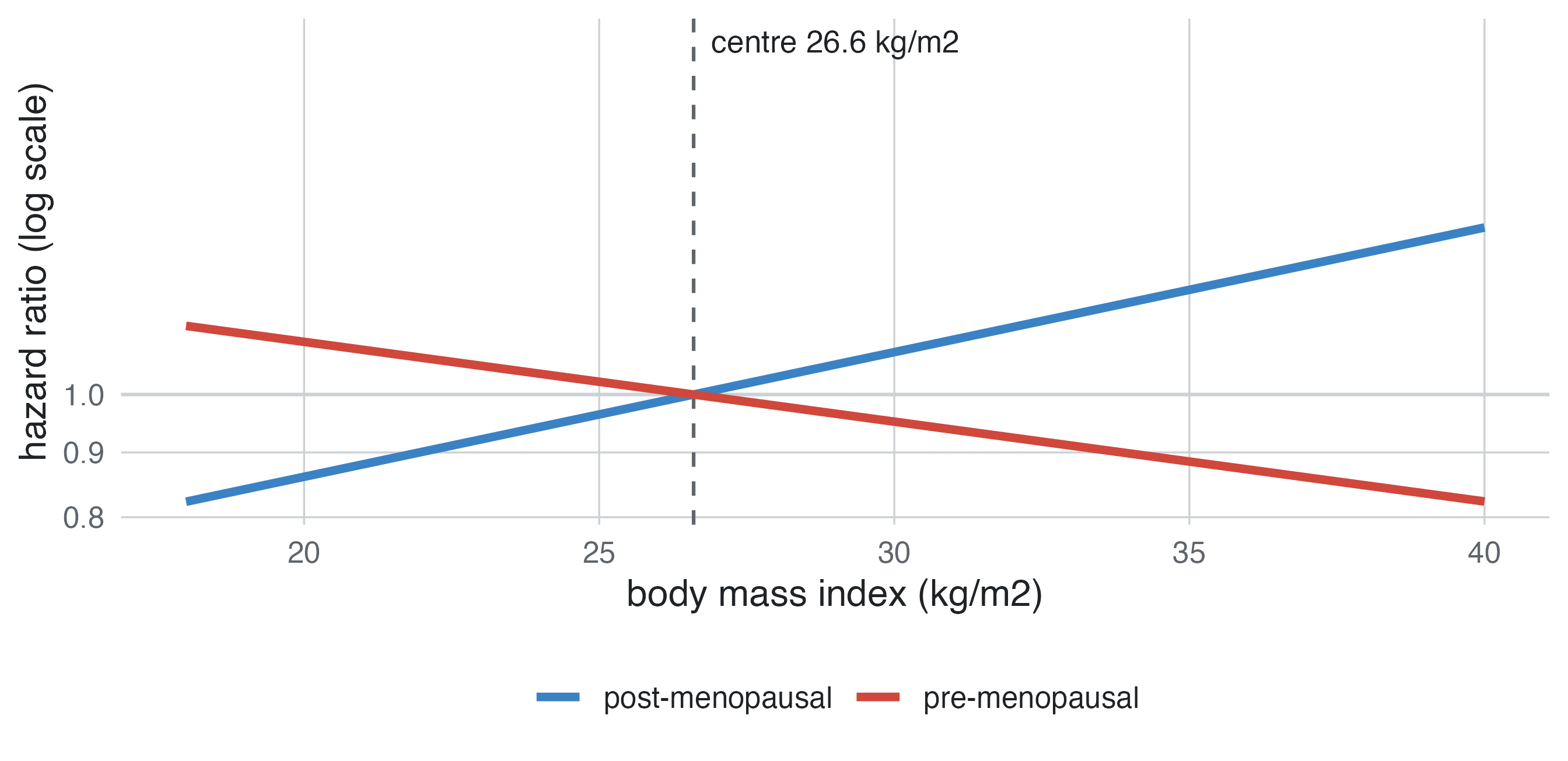
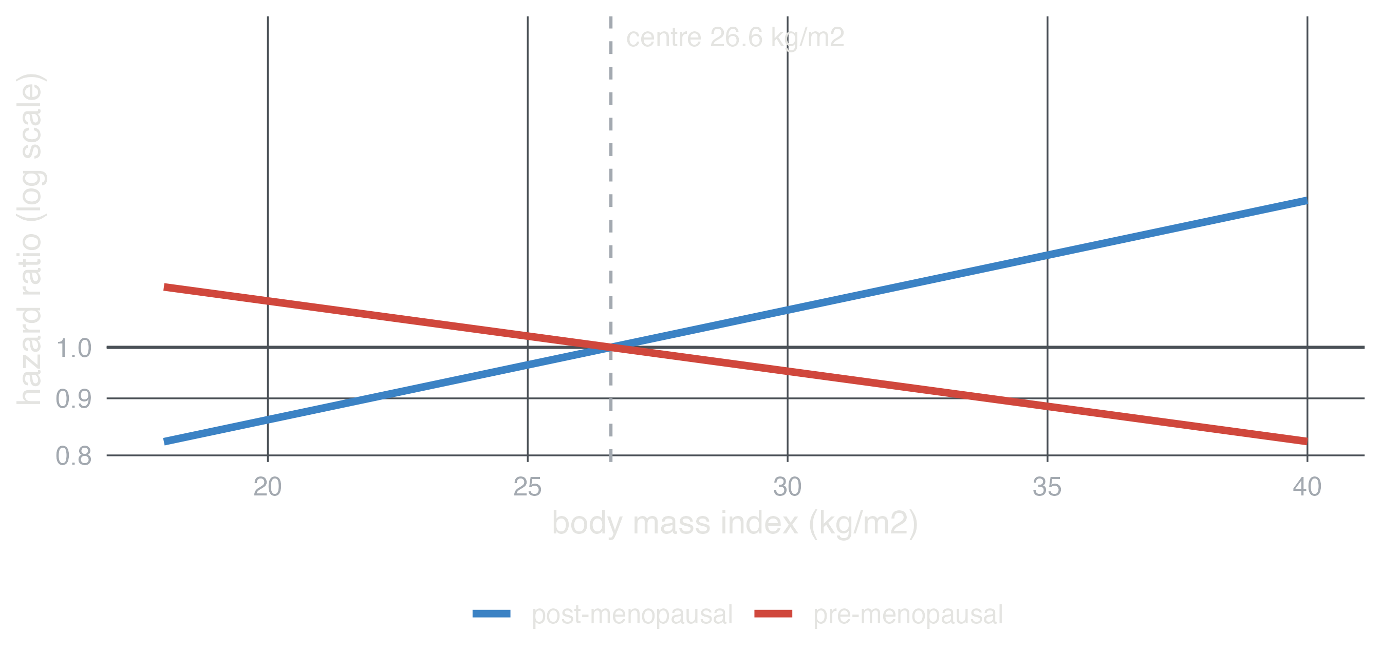
Breast cancer risk factors, case-control with two controls per case. The data are generated as a cohort with hazard ratios; the case-control odds ratios approach them because the disease is rare. Menopause is determined by age (a rule of the scenario), so much of its crude odds ratio is confounding by age. After adjustment it falls near 1, its direct effect. What remains above 1 is mediated: only post-menopausal women take hormone replacement therapy, which is not measured here, so menopause carries part of its effect (the total column). BMI’s effect, which differs before and after menopause, is centred at the population’s mean BMI, where menopause has no effect of its own.

Figure 3: Menopause has no arrow of its own into breast cancer. Age confounds it, and HRT, taken only after menopause and not measured here (dashed), mediates part of its total effect.

Variable	Contrast	True	direct	total	Crude	Adjusted (all)	Adjusted (DAG)	Estimate
age	per 1 years	HR	1.04	1.05	1.04	1.04	1.04	OR
menopause	post vs pre	HR	1.00	1.18	2.33	1.08	1.08	OR
parity	per 1 births	HR	0.93	0.93	1.02	0.94	0.94	OR
family_hist	yes vs no	HR	1.80	1.80	1.73	1.72	1.72	OR
alcohol	per 10 g/day	HR	1.07	1.07	1.08	1.08	1.08	OR

Exercise: compare with Matched case-control on age, analysed with conditional logistic regression.

Effect modification

In the same scenario BMI protects before menopause and raises risk after it. A model without the interaction gives a single, misleading BMI effect; students should fit bmi × menopause. The answer key shows the true effect per level of menopause in its note. Effect modification and interaction explains how to read the model’s coefficients, why centring BMI changes the “effect of menopause”, why the answer depends on the scale, and shows a modifier that reverses an effect (Dexamethasone in hospitalised COVID-19).

Figure 4: Effect modification is not drawn in a DAG, so here is the effect itself: the hazard ratio of breast cancer by BMI, relative to the centre, falls with BMI before menopause and rises after it.

Adjusting for everything: the Table 2 fallacy

Coronary heart disease incidence, cohort, all variables measured. Age, sex and education act partly through blood pressure, cholesterol, BMI, diabetes and HDL. A model with every variable gives their direct effects: education seems to do nothing, and the effect of sex shrinks. Adjusting each exposure only for its confounders (Adjusted (DAG)) gives the total effect, the one that answers “what if this changed?”. A single mutually adjusted table (the “Table 2” of many papers) mixes both kinds.

Figure 5: Part of the structure of Coronary heart disease incidence: age, education and sex act partly or wholly through blood pressure, smoking and HDL. A model with all of them gives the direct effects of age and sex and makes education look useless.

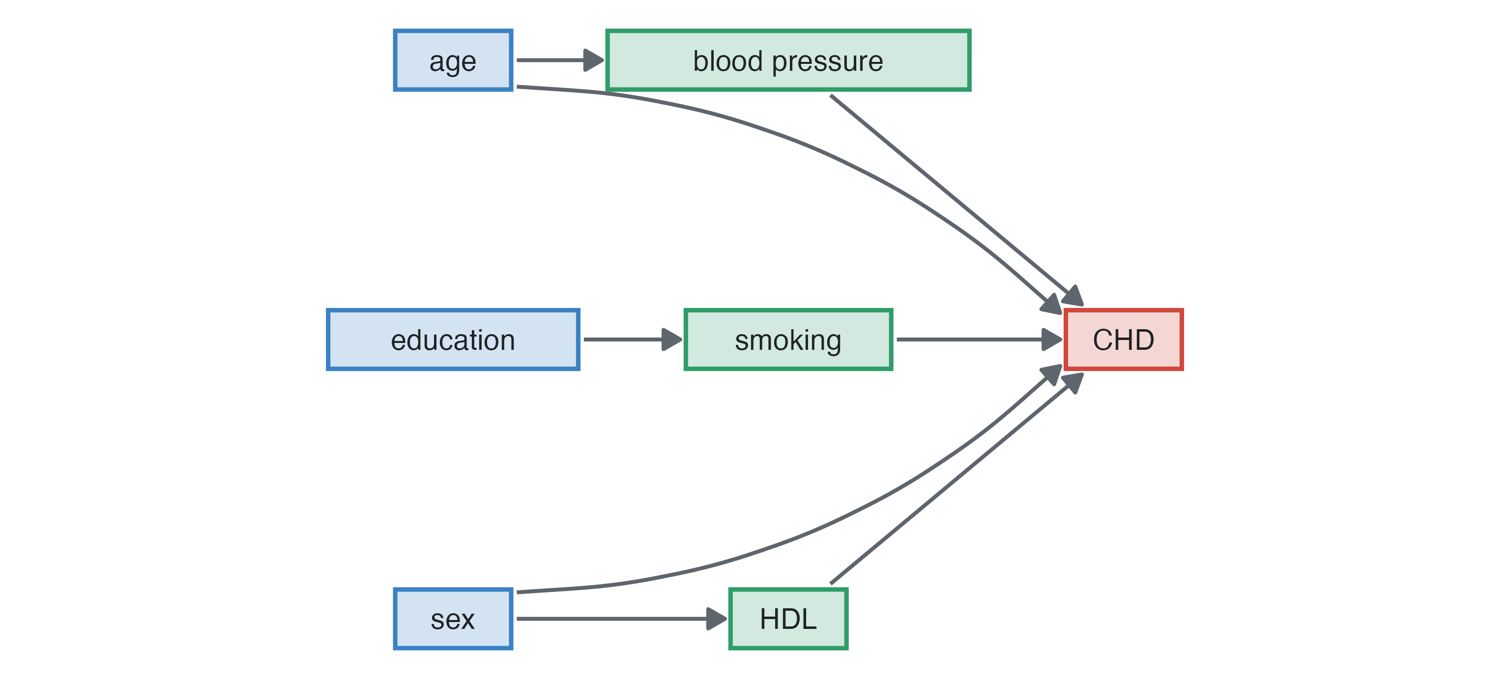
Variable	Contrast	True	direct	total	Crude	Adjusted (all)	Adjusted (DAG)	Estimate
age	per 1 years	HR	1.05	1.07	1.07	1.05	1.07	HR
sex	male vs female	HR	1.60	1.76	1.77	1.61	1.81	HR
education	secondary vs primary	HR	1.00	0.94	0.90	0.96	0.90	HR
education	university vs primary	HR	1.00	0.90	0.89	1.01	0.88	HR
total_chol	per 1 mmol/L	HR	1.20	1.20	1.31	1.20	1.20	HR
smoking	former vs never	HR	1.20	1.21	1.21	1.20	1.20	HR
smoking	current vs never	HR	1.60	1.81	1.76	1.60	1.79	HR
physical_activity	per 1 MET-h/week	HR	1.00	0.99	0.99	1.00	0.99	HR
cigarettes	per 1 cigarettes/day	HR	1.01	1.01	1.02	1.01	1.01	HR
coffee	per 1 cups/day	HR	1.00	1.00	1.08	1.01	1.01	HR
bmi	per 1 kg/m2	HR	1.02	1.06	1.07	1.02	1.06	HR
sbp	per 10 mmHg	HR	1.18	1.18	1.34	1.17	1.17	HR
hdl	per 1 mmol/L	HR	0.60	0.60	0.41	0.60	0.60	HR
diabetes	yes vs no	HR	1.80	1.80	2.94	1.88	1.88	HR

Trials: absolute effects and non-collapsibility

Rectal indomethacin to prevent post-ERCP pancreatitis, randomised trial. The key gives the risk in each arm, the risk difference and the number needed to treat. The odds ratio of the 2×2 table (the marginal one) is closer to 1 than the conditional odds ratio the data were generated with, although randomisation leaves no confounding: adjusting for prognostic variables moves it towards the conditional one.

Figure 6: In a trial nothing but randomisation causes the treatment, so there is no backdoor path. The prognostic variables (previous pancreatitis, a difficult cannulation) are precision variables: adjusting for them changes the odds ratio from marginal to conditional, not its validity.

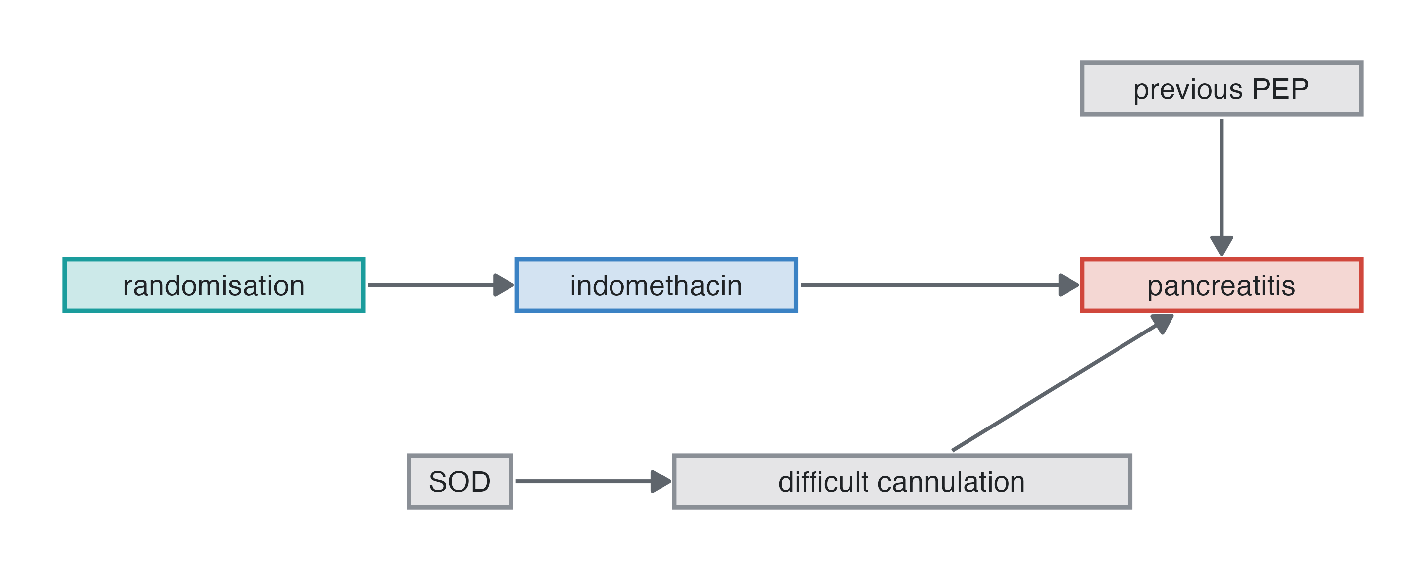
	Value
Risk: placebo	0.1700
Risk: indomethacin	0.0896
Risk difference, indomethacin vs placebo	-0.0806
Number needed to treat for one event fewer, indomethacin vs placebo	12.4000
Risk ratio, indomethacin vs placebo	0.5260
Odds ratio, marginal (population), indomethacin vs placebo	0.4800
Odds ratio, conditional (true model), indomethacin vs placebo	0.4700

Biases on purpose

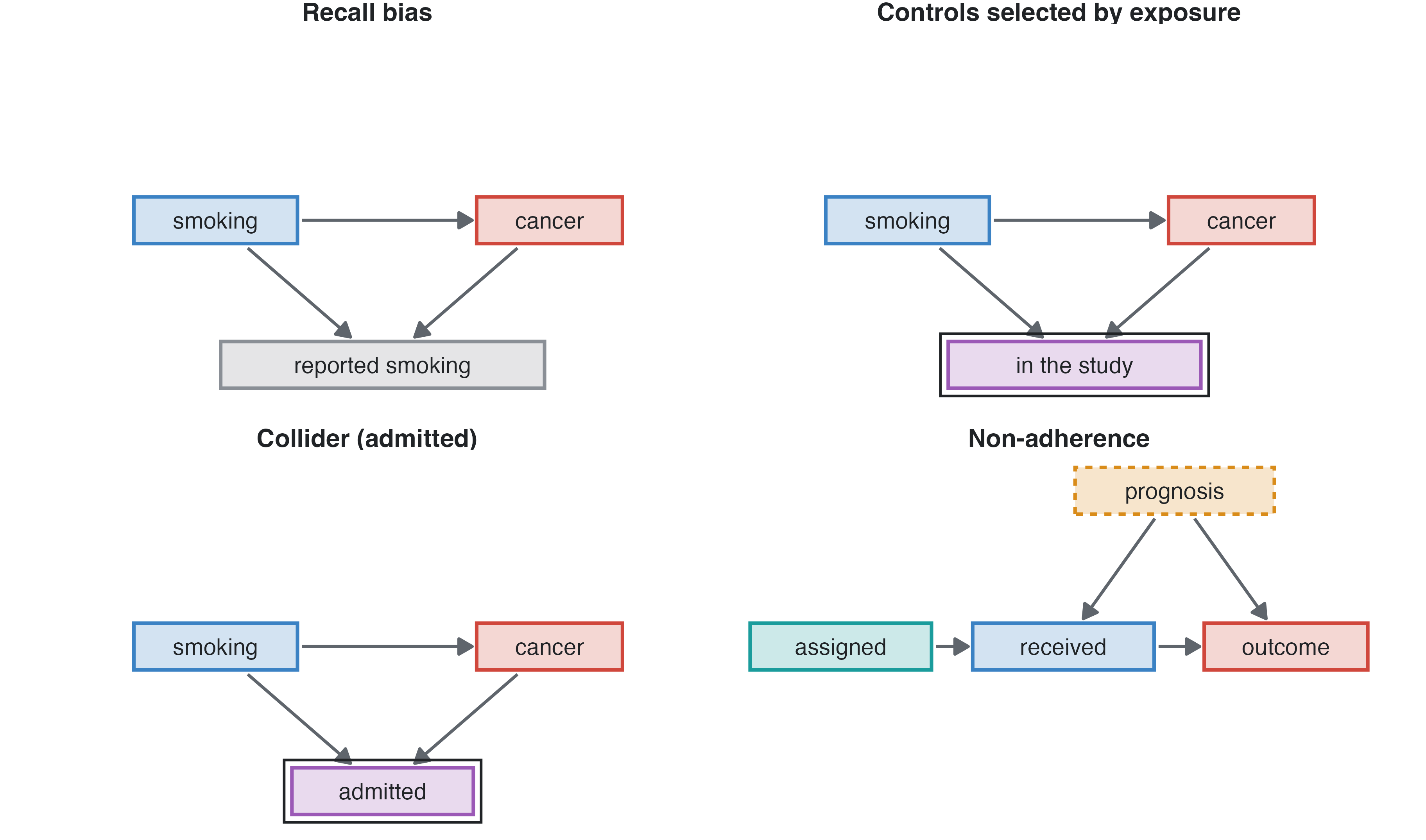
The Biases section of the panel builds a bias into the study; the answer key’s large study carries the same bias, so it shows what the biased design estimates next to the truth. Recall bias, controls selected by exposure and the collider act on the variables ticked in the Exposure column.

bias	design	what students should see
Recall bias	case-control	unexposed cases report the exposure: its odds ratio inflated
Controls selected by exposure	case-control	hospital controls with more exposure: its odds ratio towards 1
Collider (admitted)	cross-sectional, cohort, case-control	adjusting for a variable caused by the outcome and the exposure distorts the exposure’s effect
Non-adherence	randomised trial	intention to treat dilutes the effect; as treated and per protocol are confounded by prognosis
Informative loss to follow-up	followed designs	Kaplan-Meier underestimates the risk; hazard ratios shift
Immortal time	cohort, prognosis	a useless treatment started during follow-up looks protective when analysed at baseline
Spectrum, partial verification	diagnostic	sensitivity and AUC too high with severe cases; with only some negatives verified, sensitivity too high and specificity too low

Figure 7: The biases studysim can build in, as diagrams. Recall: what cases report depends on being a case. Selection and collider: the study is restricted to, or adjusted for, a variable caused by exposure and outcome (double border). Non-adherence: prognosis affects whether people take the treatment, so comparing by treatment received is confounded; by treatment assigned it is not.

Variable	Contrast	True	direct	total	Crude	Adjusted (all)	Adjusted (DAG)	Estimate
age	per 1 years	HR	1.09	1.09	1.09	1.09	1.09	OR
sex	male vs female	HR	1.20	2.46	2.70	1.21	2.72	OR
smoking	former vs never	HR	4.00	4.00	7.87	7.66	7.66	OR
smoking	1-14 vs never	HR	7.70	7.70	12.01	11.43	11.43	OR
smoking	15-24 vs never	HR	13.70	13.70	21.87	20.19	20.19	OR
smoking	25+ vs never	HR	24.50	24.50	41.97	37.87	37.87	OR

Recall bias of 30% on smoking (lung cancer, case-control): every smoking odds ratio is inflated.

Chance and bias: replicate studies

Compare designs with 200 replicate studies per design: the spread of the estimates is the standard error a single study only estimates; a confidence interval should contain the true value in about 95% of the studies, and power is the share of studies that find the effect. A biased design shows a shifted distribution and poor coverage, however many studies are drawn.

Categorising a continuous variable

Systolic pressure in quartiles (Form: quartiles) gives a dose-response pattern but loses information: compare the precision of the per-10-mmHg estimate with the quartile contrasts, and the effect of choosing other cut points.

Variable	Contrast	True	direct	total	Crude	Adjusted (all)	Adjusted (DAG)	Estimate
age	per 1 years	HR	1.05	1.07	1.07	1.06	1.07	HR
sex	male vs female	HR	1.60	1.76	1.77	1.79	1.79	HR
sbp	Q2 vs Q1	HR	NA	NA	1.58	1.32	1.32	HR
sbp	Q3 vs Q1	HR	NA	NA	2.30	1.67	1.67	HR
sbp	Q4 vs Q1	HR	NA	NA	3.74	2.30	2.30	HR

Trials: parallel and crossover

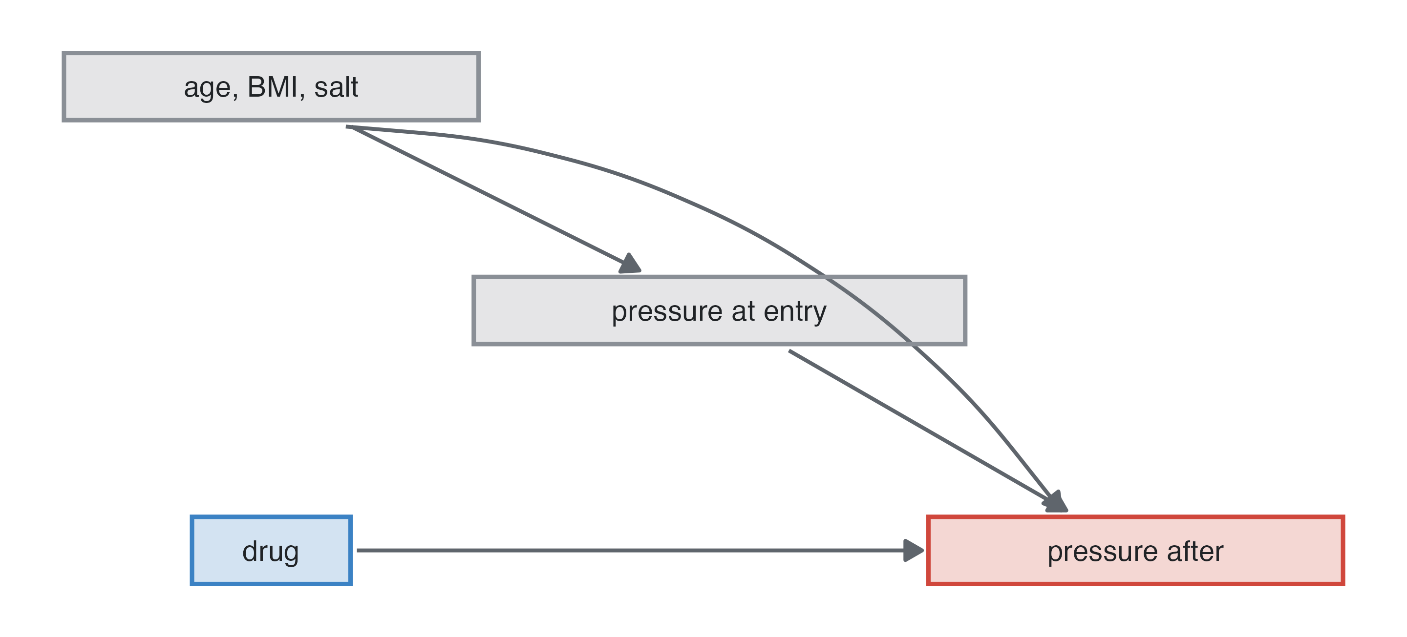
Antihypertensive drug vs placebo: in the parallel trial the unadjusted difference is unbiased, and adjusting for baseline pressure (ANCOVA) narrows the interval. In the 2×2 crossover each patient is their own control: 30 patients give a precise estimate, and the period effect must be in the model.

Figure 8: A parallel trial: the pressure at entry predicts the pressure after treatment but is not caused by the drug. It is a precision variable, and adjusting for it (ANCOVA) narrows the interval without changing what is estimated.

Variable	Contrast	True	direct	Crude	Adjusted (all)	Estimate
drug	amlodipine vs placebo	beta	-9	-8.99	-8.97	beta

Variable	Contrast	True	direct	Crude	Adjusted (all)	Estimate
drug	amlodipine vs placebo	beta	-9	-8.92	-8.92	beta

Bioequivalence of two formulations: AUC and Cmax are log-normal; analyse log values and back-transform to a geometric mean ratio, then check whether its 90% CI lies within 0.80–1.25.

Assignments with student keys

Give every student the same options and their own student key (e.g. their ID): each gets a different dataset from the same superpopulation. The teacher reproduces any of them by typing the key, and the answer key is the same for all.

Export class (Output) does it in one go: type the student keys (separated by commas) and it saves a zip with one CSV and one codebook per student, a register of keys and seeds, and one answer key report. Students then get only their data.

A teacher code keeps the key out of the students’ panel: typed in Library before exporting a library, it locks that library; while it is loaded, the answer key, its report, the class export, the effect sizes on the diagram, the true values of Compare designs and the effects in Library need the code. It is a deterrent, not protection: the library file itself holds the parameters. The causal diagram is shown without effect sizes by default.