

Epidemiology guide, part 1
Every analysis in this guide goes through the same steps. A question (“does smoking cause coronary heart disease, and by how much?”) becomes an estimand: a precise quantity, such as the risk ratio of a 10-year coronary event for smokers against non-smokers with the same age and sex. A design gathers data that can estimate it. A causal diagram says which variables to adjust for. A model turns the data into a number, and the number is interpreted on the scale of the estimand. This page covers the last two steps: the measures epidemiology uses and how the coefficients of its models are read. The next pages cover the designs, the diagrams and mediation (Lash et al. 2021; Hernán and Robins 2020).
| measure | definition | example | typical design |
|---|---|---|---|
| Prevalence | proportion of a population that has the condition at a time | 18% of adults have hypertension | cross-sectional |
| Risk (cumulative incidence) | proportion of people free of the outcome at the start who develop it over a period | 8% have a coronary event in 10 years | cohort, trial |
| Rate (incidence density) | new cases per unit of person-time | 2.5 breast cancers per 1000 woman-years | cohort |
| Odds | probability / (1 − probability) | a risk of 0.2 is odds of 0.25 | case-control (only odds ratios) |
| Hazard | instantaneous rate among those still at risk at a given time | cohort with times (Cox) |
Prevalence mixes how often a condition starts and how long it lasts: in a steady population, prevalence ≈ incidence rate × mean duration. A treatment that keeps patients alive longer raises prevalence. A risk always refers to a period (“10-year risk”), and it requires everyone to be followed for that period or a method that handles censoring (Kaplan-Meier). When another event can prevent the outcome (death from other causes before a cancer relapse), the risk of the outcome is a cumulative incidence in the presence of a competing event. One minus Kaplan-Meier, which censors the competing deaths, overstates it.
| measure | definition | estimated by |
|---|---|---|
| Risk difference (RD) | risk1 − risk0 | cohort, trial (2×2 table, binomial model with identity link) |
| Number needed to treat (NNT) | 1 / |RD| | trial |
| Risk ratio (RR) | risk1 / risk0 | cohort, trial, cross-sectional (prevalence ratio) |
| Rate ratio (IRR) | rate1 / rate0 | cohort (Poisson regression with log person-time as offset) |
| Hazard ratio (HR) | hazard1 / hazard0, assumed constant over time | cohort, trial (Cox regression) |
| Odds ratio (OR) | odds1 / odds0 | any design; the only one a case-control study gives |
| Mean difference | mean1 − mean0 | linear regression |
| Ratio of geometric means | exp(mean of log1 − mean of log0) | linear regression of a log outcome |
Difference measures say how many people are affected, and that is what decisions need. Ratio measures say how strong the association is, and they are usually more stable across populations with different baseline risks. Report both when you can: a risk ratio of 2 means 10 extra cases per 1000 people if the baseline risk is 1%, and 200 if it is 20%.
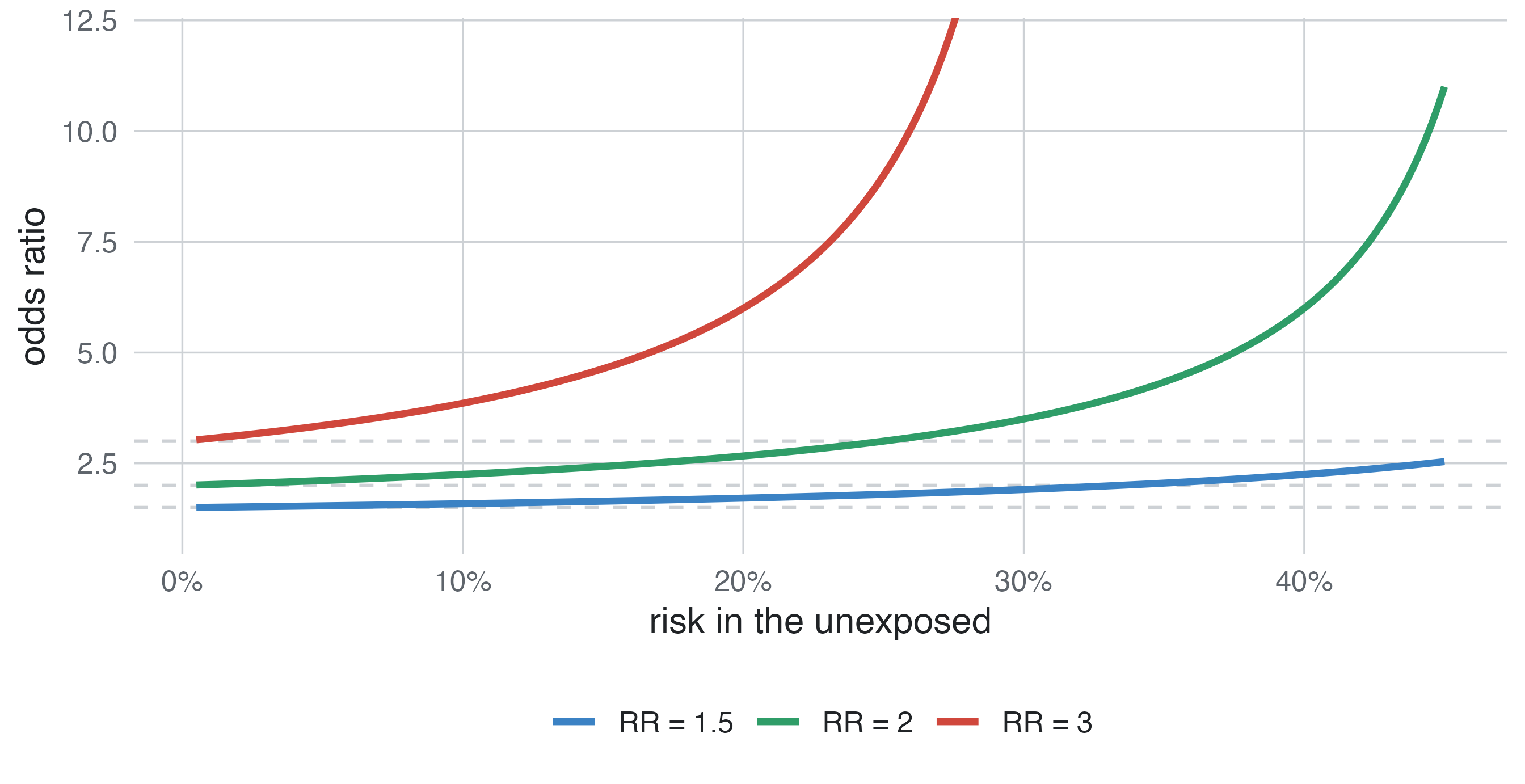
The odds ratio approaches the risk ratio only when the outcome is rare (Figure 2). A case-control study of a rare disease therefore estimates the risk (or rate) ratio. A cross-sectional study of a common condition analysed with logistic regression reports odds ratios that look much stronger than the prevalence ratios.
The odds ratio and the hazard ratio have a property that surprises many people. Suppose a treatment multiplies the odds by 3 in every subgroup of patients and the subgroups are perfectly balanced between the arms, so nothing is confounded. The odds ratio of the whole trial is still smaller than 3 (Greenland et al. 1999). Risk differences and risk ratios do not behave this way.
| risk, control | risk, treated | OR | RR | RD | |
|---|---|---|---|---|---|
| low risk | 0.10 | 0.250 | 3.00 | 2.50 | 0.150 |
| high risk | 0.60 | 0.818 | 3.00 | 1.36 | 0.218 |
| whole population (half each) | 0.35 | 0.534 | 2.13 | 1.53 | 0.184 |
Both subgroups have an odds ratio of 3, and the whole population has 2.13. Neither number is wrong: they answer different questions. The conditional odds ratio is the effect for a patient with given characteristics; the marginal one is the effect on the population. In a trial the crude analysis estimates the marginal effect and an analysis adjusted for prognostic variables the conditional one, which is further from 1. studysim generates data with conditional effects, and its answer key shows both for trials (absolute effects in the trial).
| Value | |
|---|---|
| Risk: placebo | 0.1700 |
| Risk: indomethacin | 0.0896 |
| Risk difference, indomethacin vs placebo | -0.0806 |
| Number needed to treat for one event fewer, indomethacin vs placebo | 12.4000 |
| Risk ratio, indomethacin vs placebo | 0.5260 |
| Odds ratio, marginal (population), indomethacin vs placebo | 0.4800 |
| Odds ratio, conditional (true model), indomethacin vs placebo | 0.4700 |
| outcome | model | exp(β) or β is | jamovi |
|---|---|---|---|
| continuous | linear regression | β: difference in the mean per unit of x | Regression ▸ Linear Regression |
| continuous, skewed | linear regression of log(y) | exp(β): ratio of geometric means | Compute log(y), then linear regression |
| binary | logistic regression | odds ratio | Regression ▸ Logistic Regression ▸ 2 Outcomes |
| binary, matched sets | conditional logistic regression | odds ratio within sets | condLogReg |
| count or rate | Poisson (negative binomial) regression, log person-time as offset | rate ratio | GAMLj |
| time to event | Cox regression | hazard ratio | prognosis |
The same rules apply to every model:
center: solves in its own scenarios.| column | estimand |
|---|---|
| Direct (conditional) | the effect in the generating model, every other variable fixed |
| Total | the effect of changing the variable while its consequences change too, given the variables it does not cause (Causal diagrams) |
| Crude | the association without adjustment |
| Adjusted (all) | the conditional association given every measured variable |
| Adjusted (DAG) | the association given the measured variables that the diagram says to adjust for |
| Absolute effects (trials) | risks per arm, RD, NNT, marginal and conditional OR or HR |
They are estimated the same way (X within levels of Z, or a product term X × Z), and the words are often used interchangeably. The distinction matters when deciding what to do: a modifier tells you who benefits most from acting on X.
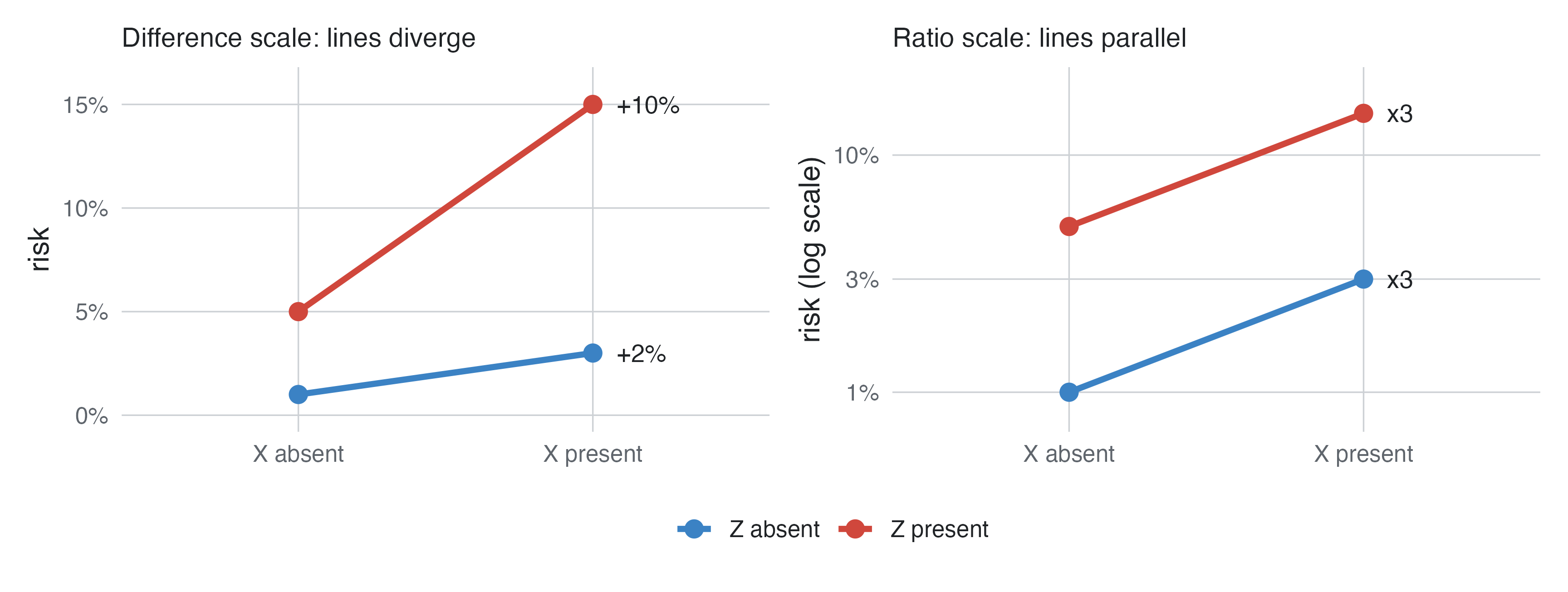
Whether an effect “differs” depends on how effects are measured. In this example, exposure X triples the risk both in people without and with a second factor Z:
| risk, X absent | risk, X present | risk ratio of X | risk difference of X | |
|---|---|---|---|---|
| Z absent | 1% | 3% | 3 | +2% |
| Z present | 5% | 15% | 3 | +10% |
On the ratio scale there is no modification: the risk ratio is 3 in both groups. On the difference scale there is a great deal: X adds 2 cases per 100 people without Z and 10 per 100 with Z (Figure 3). Whenever two factors both act, no modification on one scale implies modification on the other.
Logistic and Cox models are multiplicative: their product term tests departure from multiplying the effects. Public health usually cares about the additive scale, because it counts cases: here, removing X prevents five times more cases among people with Z. The relative excess risk due to interaction, RERI = RR11 − RR10 − RR01 + 1, measures additive interaction from ratio measures: here 15 − 3 − 5 + 1 = 8 (0 means no additive interaction).
In a model logit(risk) = β0 + β1·X + β2·Z + β3·X·Z:
| coefficient | is | holds |
|---|---|---|
| exp(β1) | odds ratio of X | when Z = 0 (its reference level) |
| exp(β2) | odds ratio of Z | when X = 0 |
| exp(β3) | ratio of the odds ratios of X between Z = 1 and Z = 0 | the multiplicative interaction |
| exp(β1 + β3) | odds ratio of X | when Z = 1 |
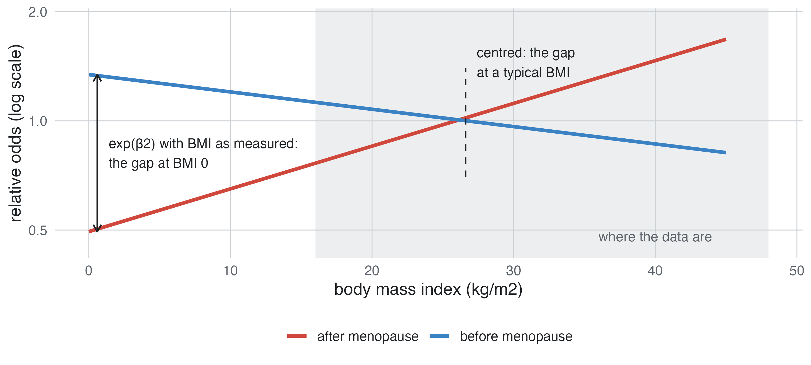
The “main effects” are therefore not average effects: each is the effect at the reference or zero of the other variable. When the other variable is continuous and zero is meaningless, a main effect is an extrapolation far from the data. Centre the continuous variable first (subtract a typical value), so that the main effect of the modifier holds at that typical value.
Breast cancer risk factors: the effect of BMI is modified by menopause (per 5 kg/m², HR 0.93 before and 1.12 after). The table fits the same interaction model to a large simulated case-control study, with BMI as it is and centred at the population mean.
| BMI as measured | BMI centred at 26.6 | |
|---|---|---|
| BMI per 5 kg/m², before menopause (exp β1) | 0.95 | 0.95 |
| BMI per 5 kg/m², after menopause (exp(β1 + β3)) | 1.15 | 1.15 |
| ratio of the two (exp β3) | 1.21 | 1.21 |
| menopause, post vs pre (exp β2) | 0.37 | 1.02 |
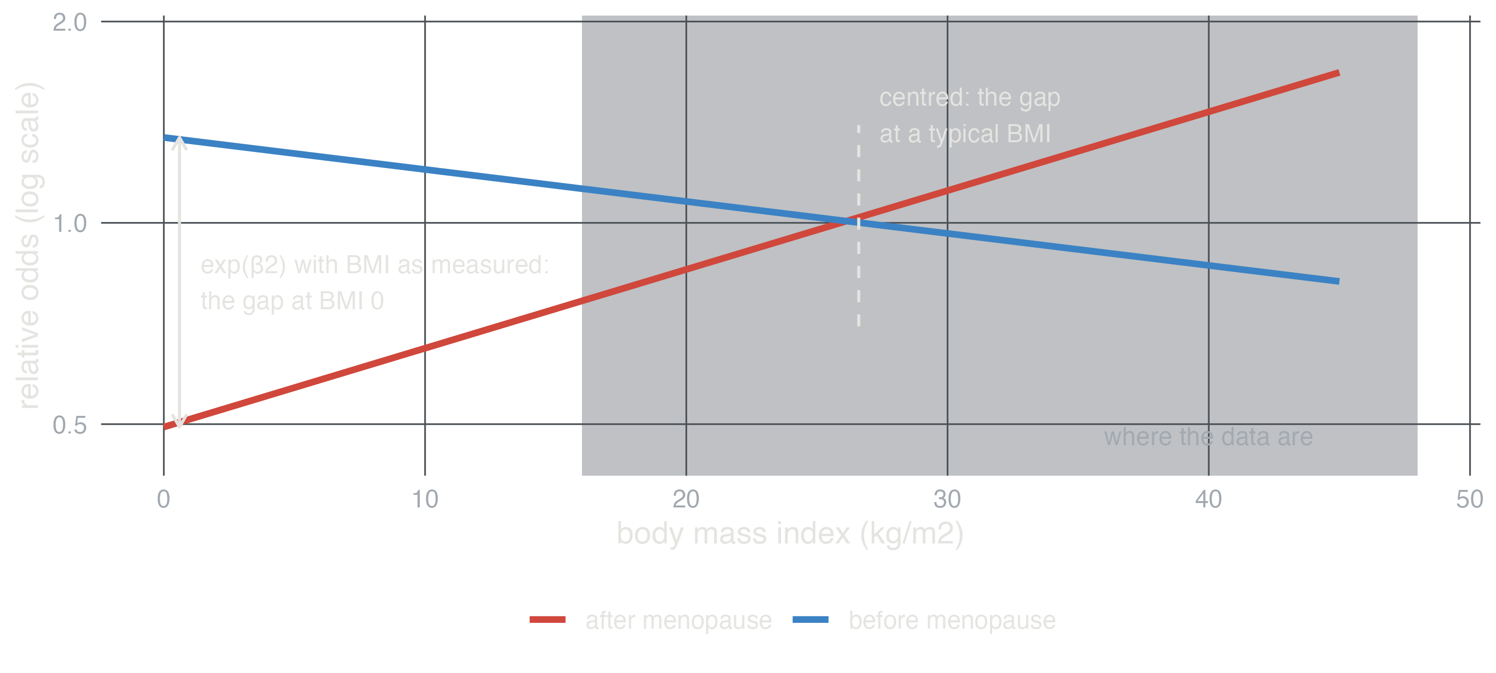
The BMI effects and their ratio do not change with centring. The “effect of menopause” does: with BMI as measured it is the odds ratio at a BMI of 0, which nobody has (Figure 4). Centred, it is the odds ratio at a typical BMI, which is what the question means.
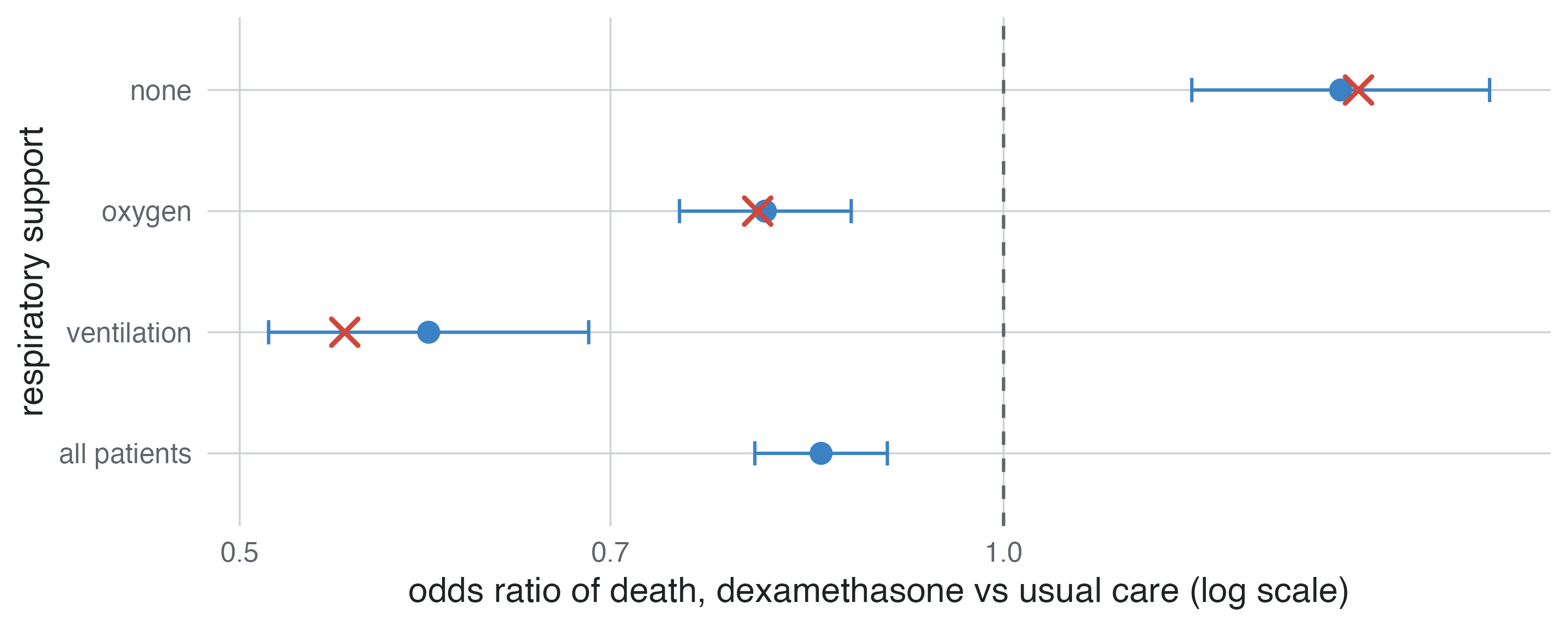
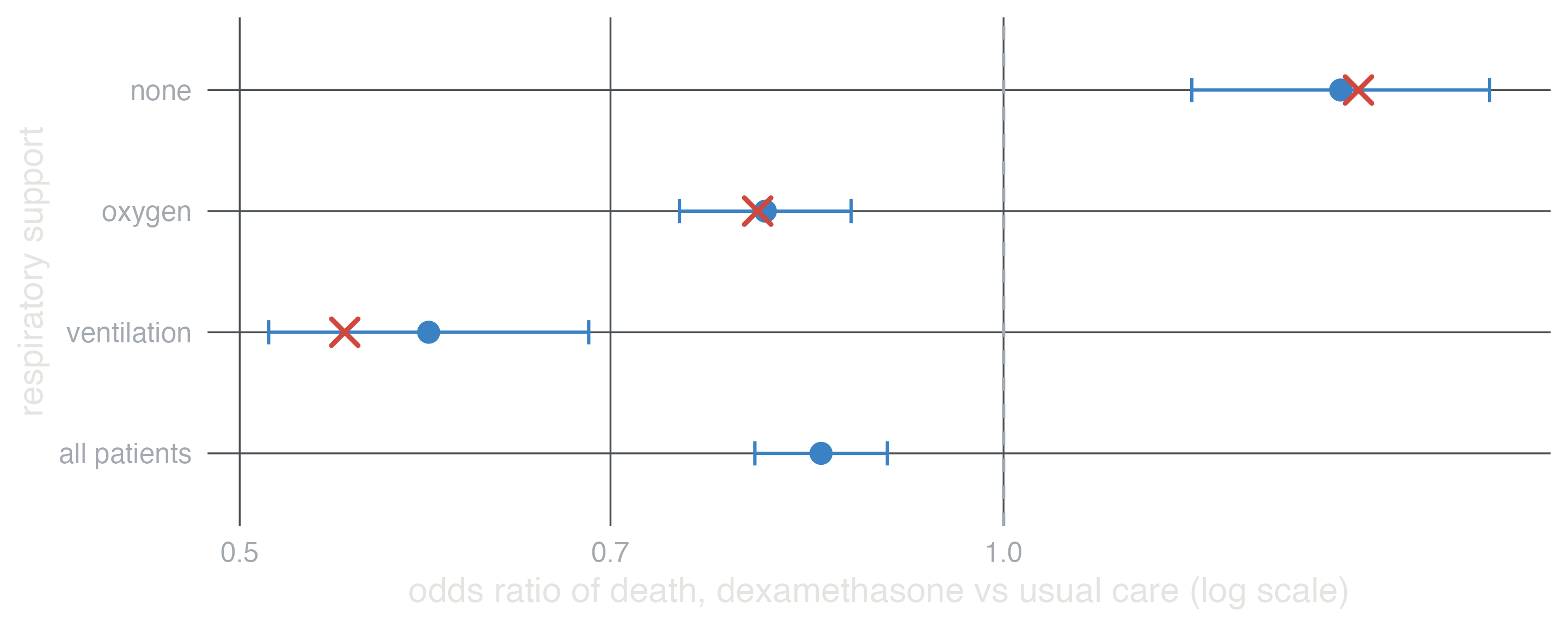
Dexamethasone in hospitalised COVID-19 (RECOVERY): dexamethasone lowers mortality in patients on oxygen or ventilation, but not in those without respiratory support. This is qualitative modification: the effect changes direction. Its overall odds ratio, averaged over the patients of the trial, would hide both the harm and the largest benefit.
In jamovi: in Regression models, select both variables in Model Builder and add their interaction (centre a continuous modifier first with Compute); Frequencies ▸ Independent Samples with the modifier as Layer gives the odds ratio in each group and a test of homogeneity; the prognosis module gives subgroup hazard ratios for an interaction in a Cox model, and GAMLj simple effects. In studysim: Breast cancer risk factors (BMI × menopause), Dexamethasone in hospitalised COVID-19 (treatment × respiratory support), HPV and cofactors of cervical cancer (IARC multicentric) (cofactors that act only with HPV), and the 2×2 factorial design with an interaction between the two treatments.