Regression is used for two different purposes. In an aetiological study the question is the effect of one exposure, and the other variables are there to remove confounding: the coefficient of the exposure is the result. In a prediction study no coefficient is the result: the result is the predicted risk of each patient, and the question is whether these risks are accurate (calibration) and separate patients with and without the outcome (discrimination) in patients who were not used to build the model (Steyerberg 2019). A predictor need not be causal; it must only carry information that is available at the moment of prediction.
A diagnostic model predicts the presence of a disease now (e.g. pulmonary embolism in a patient with chest pain); a prognostic model predicts a future event (e.g. a cardiovascular event within 10 years). The tools are the same.
clinpred covers steps 3 to 9.
A model fitted to a data set describes that data set best, noise included. Its apparent performance, measured in the same patients, is therefore optimistic: in new patients the discrimination will be lower and the predictions too extreme (high risks too high, low risks too low). The more parameters relative to the number of events, the larger the optimism.
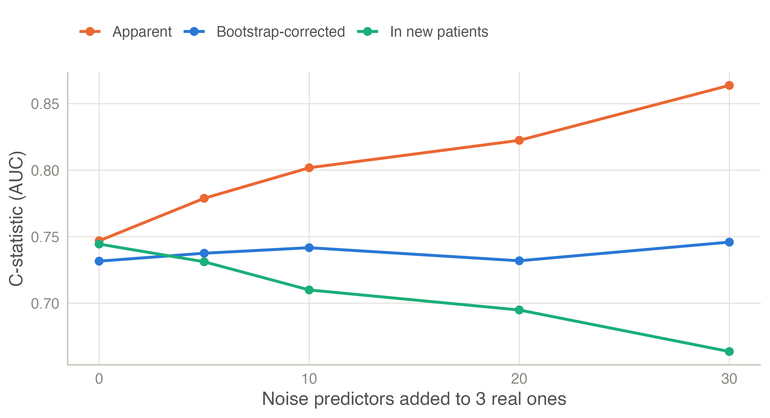
The simulation below shows it. Each data set has 300 patients (about 45 events) and three real predictors; noise predictors are then added. The apparent C-statistic (AUC) keeps rising with every useless predictor, while the AUC in a large independent sample falls. The bootstrap optimism-corrected AUC, computed by clinpred’s own validation engine, removes most of the optimism. It removes less of it when the parameters approach the number of events: there the data are too few even to estimate the optimism, which is one more reason to respect the sample size (below).
With 30 noise predictors (33 parameters for about 45 events) the apparent AUC is 0.864, but in new patients it is 0.664; the bootstrap says 0.746. The bootstrap also estimates how much the predictions are too extreme: the calibration slope of the model in new patients, 0.43 here (1 would be perfect). This is the uniform shrinkage factor: multiplying the coefficients by it would make the predictions about right. The validation page explains how the bootstrap does this.
The remedies are, in order: fewer candidate parameters (pre-specification from knowledge), more data, and penalised estimation (shrinkage, elastic net). Selection by p-values or AIC does not remove the optimism — it adds its own — unless it is repeated inside the validation, as clinpred does.
The old rule of 10 events per variable is too crude. Riley et al. (2020) (and Richard D. Riley et al. (2019a), Richard D. Riley et al. (2019b) for continuous and time-to-event outcomes) derive the minimum sample size from explicit targets:
The criteria depend on the number of candidate parameters (every spline term, every factor level, every candidate interaction counts, whether or not it is kept), the outcome proportion, and the anticipated Cox–Snell R² of the model. clinpred’s Sample size adequacy table computes the three criteria from the anticipated R² you enter or from the model’s own optimism-corrected R², and compares them with the data you have (see the logistic example).