A prediction model is judged on four aspects (Steyerberg et al. 2010). None of them replaces the others: a model can rank patients well and still give wrong risks, or give right risks that change no decision.
| Aspect | Question | Main measures in clinpred |
|---|---|---|
| Discrimination | Do patients with the outcome get higher predictions? | C-statistic (AUC); Harrell’s and Uno’s C, time-dependent AUC (Cox) |
| Calibration | Are the predicted risks right? | calibration-in-the-large, calibration slope, O/E, ICI, calibration plot |
| Overall | How close are predictions to outcomes? | Brier score, scaled Brier, R² (Nagelkerke, Cox–Snell; R², RMSE, MAE for linear) |
| Clinical utility | Does using the model improve decisions? | net benefit, decision curves; sensitivity, specificity at a threshold |
The examples on this page use the logistic model of the heart cohort (age as a spline with an age × sex interaction, blood pressure, cholesterol, smoking and diabetes): 2360 patients, 364 of whom had a cardiovascular event within 10 years (15.4%).
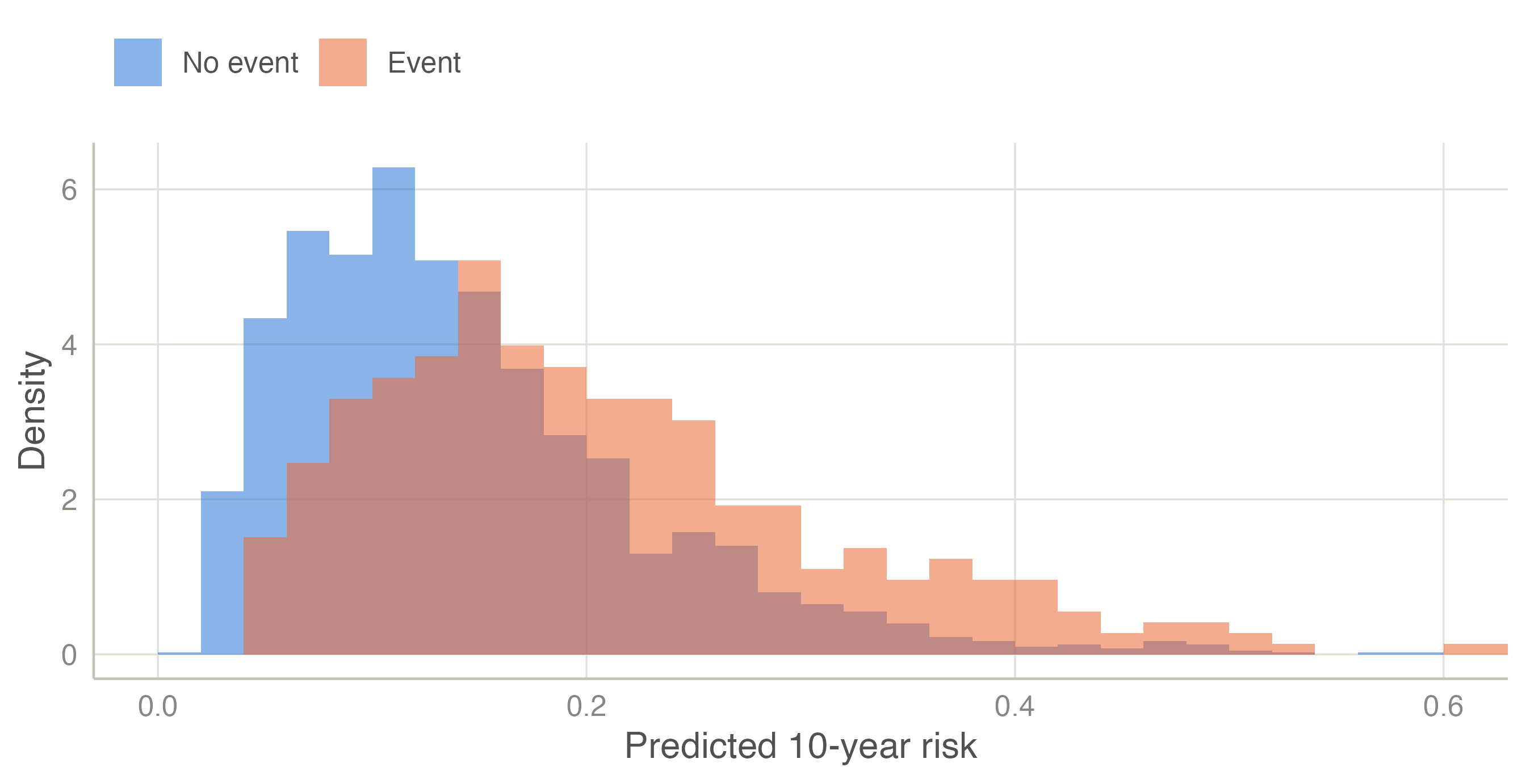
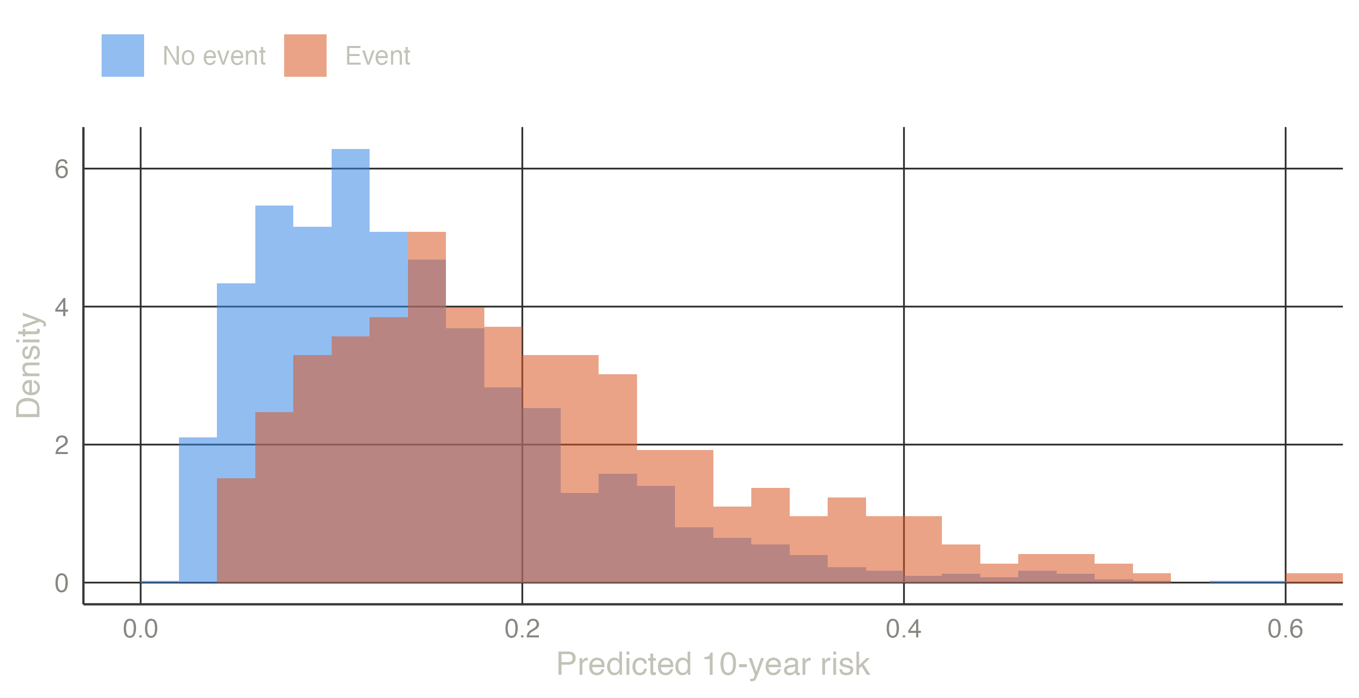
A model discriminates if it gives higher risks to the patients who will have the event than to those who will not. Look at the predicted risks of the two groups:
Patients with an event tend to have higher predicted risks (median 19% against 13%), but the distributions overlap widely: many patients without an event get higher risks than some with one. The C-statistic puts a number on this overlap.
Take one patient with the event and one without. If the model gave the higher risk to the patient with the event, the pair is concordant; otherwise it is discordant (a tie counts half). The C-statistic is the proportion of concordant pairs among all such pairs. With 4 patients with an event and 5 without there are 4 × 5 = 20 pairs:
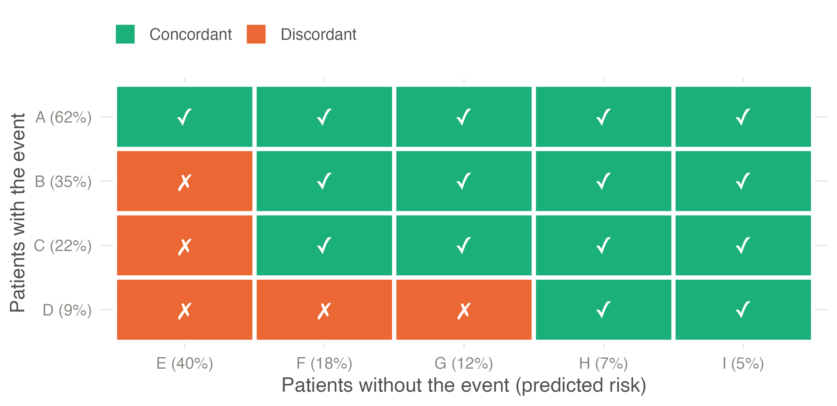
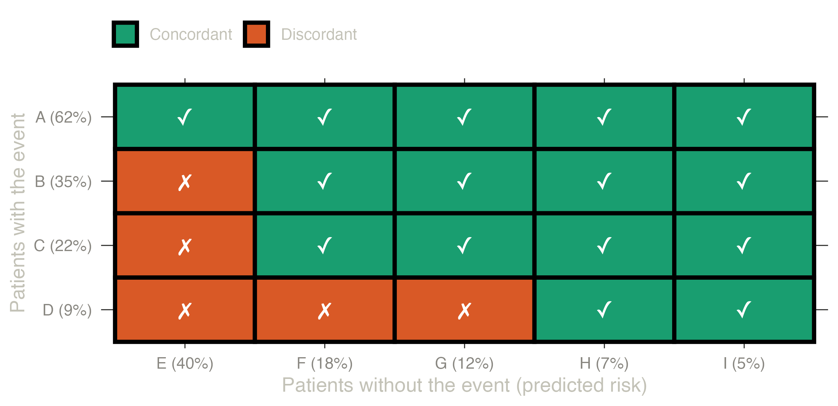
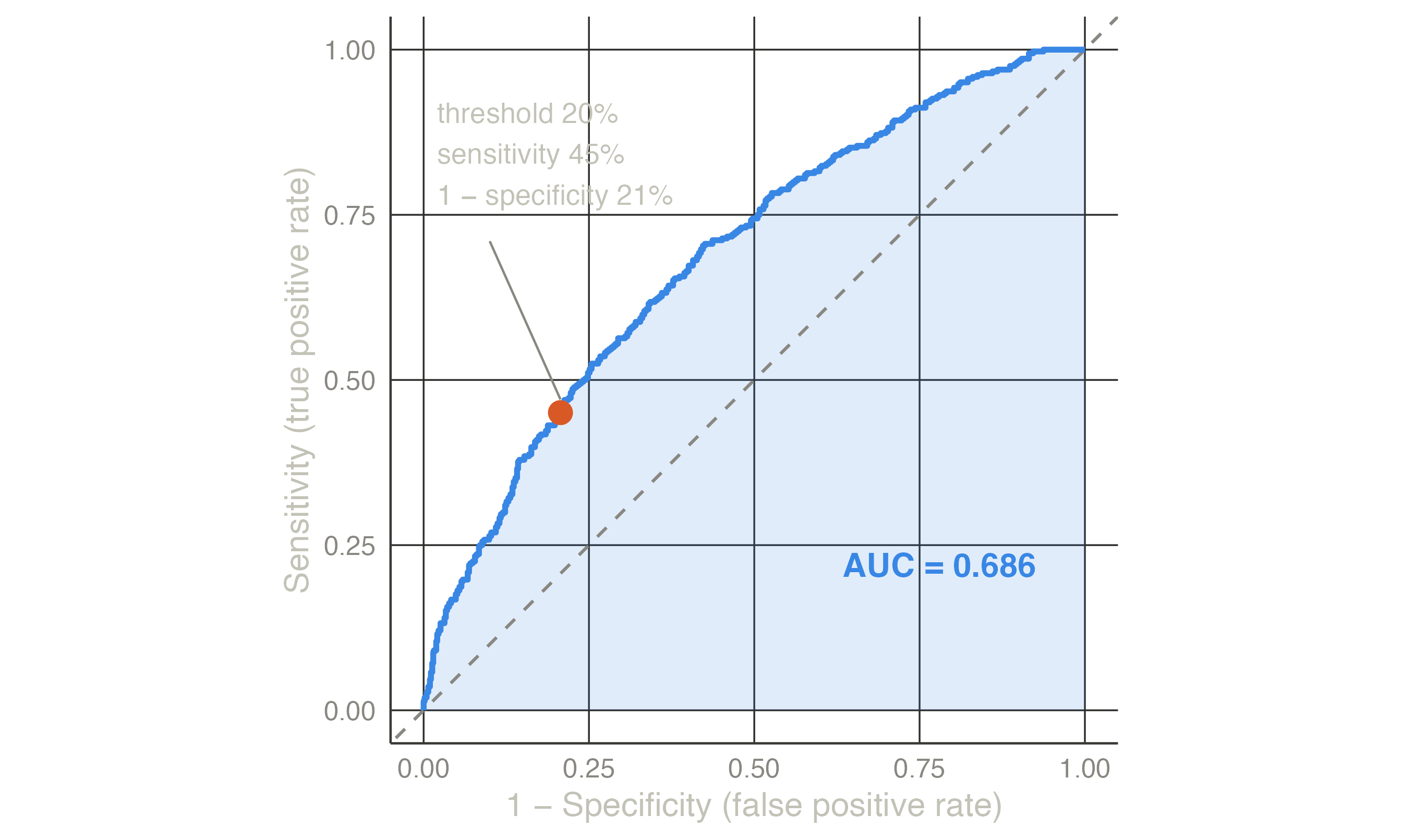
Patient A (risk 62%) is ranked above every patient without the event; patient D (9%) above only two of them. 15 of 20 pairs are concordant, so C = 0.75: for a random pair, the model ranks the patient with the event higher 75% of the time. For the heart model the same count over all 364 × 1996 = 726,544 pairs gives C = 0.686.
How to read it: 0.5 is a coin toss (the model ranks no better than chance), 1 is perfect separation. 0.7–0.8 is typical of clinical models built from routine variables; above 0.8 is good. The C-statistic says nothing about whether the risks are right: doubling every risk would not change a single pair.
For a binary outcome the C-statistic equals the area under the ROC curve (AUC). Choose a threshold — treat everyone above 20% — and count how many patients with the event are above it (sensitivity) and how many without the event are wrongly above it (1 − specificity). Each threshold gives one point; joining all of them, from 100% (nobody above) to 0% (everyone above), draws the ROC curve.
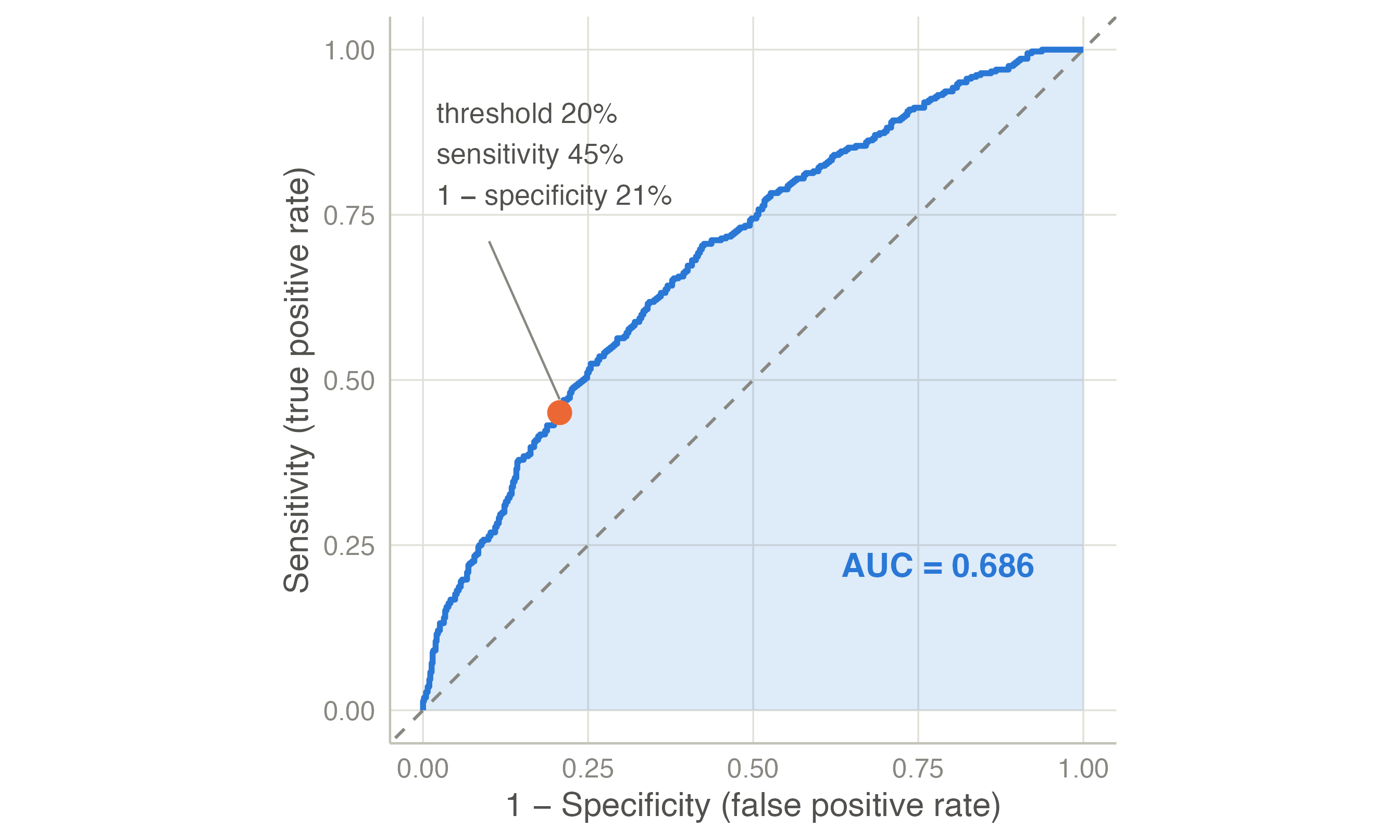
For time-to-event outcomes, Harrell’s C compares the pairs whose order of events is known (the one who had the event first should have the higher risk); Uno’s C weights the pairs for censoring and restricts them to the horizon (Uno et al. 2011); the time-dependent AUC separates the patients with an event by the horizon from those event-free at it. Royston’s D measures the separation of the prognostic index (Royston and Sauerbrei 2004). clinpred gives DeLong’s confidence interval for the AUC (DeLong et al. 1988).
Discrimination depends on the case-mix: in a population where patients differ more, the same model discriminates better. Comparing AUCs across populations needs care (see the external validation example).
Calibration is the agreement between predicted risks and observed frequencies: among patients given a 20% risk, about 20% should have the event. It is the aspect most often neglected — “the Achilles heel of predictive analytics” (Van Calster et al. 2019) — and a miscalibrated model misleads every patient it is used on, whatever its AUC.
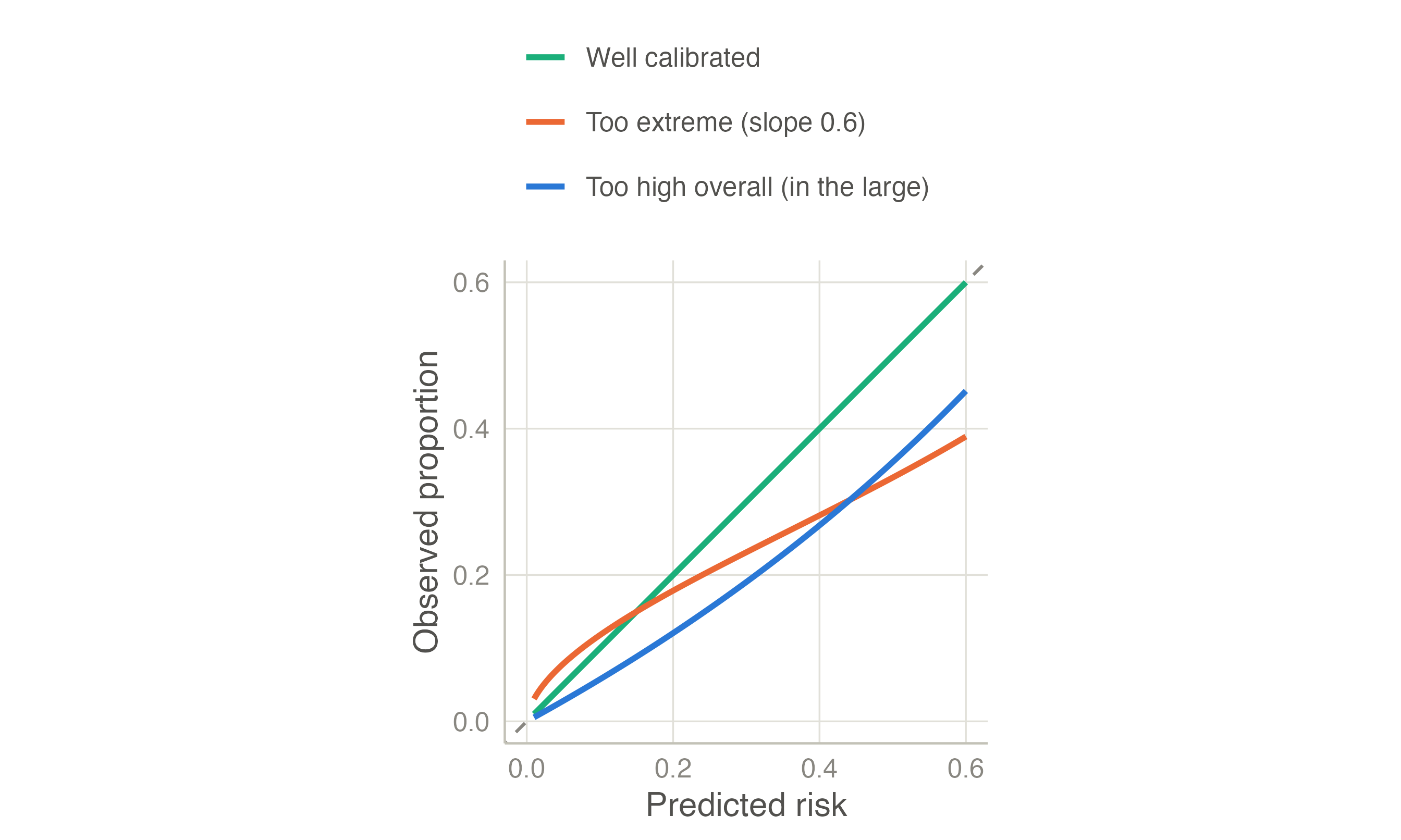
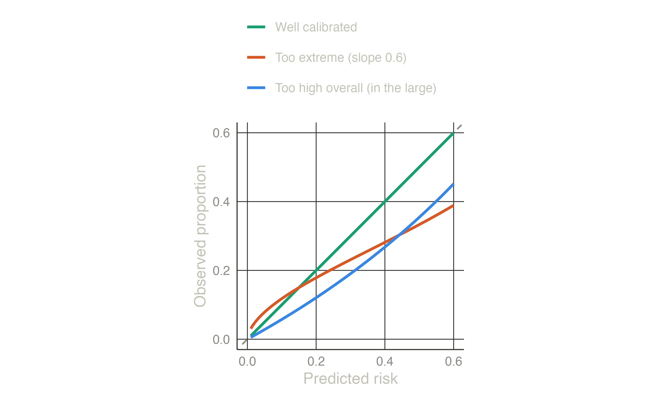
The measures follow a hierarchy (Van Calster et al. 2019):
The Brier score asks, patient by patient, how far the predicted risk was from what happened. What happened is coded 1 (event) or 0 (no event); the error is the difference, squared so that errors in both directions count, and averaged over patients:
\[\text{Brier} = \frac{1}{N}\sum_{i=1}^{N} (\text{outcome}_i - \text{predicted risk}_i)^2.\]
| Patient | Predicted risk | Outcome | Squared error |
|---|---|---|---|
| 1 | 0.0500 | 0 | 0.0025 |
| 2 | 0.1000 | 0 | 0.0100 |
| 3 | 0.2000 | 1 | 0.6400 |
| 4 | 0.3000 | 0 | 0.0900 |
| 5 | 0.6000 | 1 | 0.1600 |
| 6 | 0.8000 | 1 | 0.0400 |
Patient 1 was given 5% and had no event: a tiny error (0.0025). Patient 3 was given 20% and had the event: a large error (0.64). The Brier score of these six is the mean of the last column, 0.157. Lower is better; 0 would be a model that predicts 0% for everyone without the event and 100% for everyone with it.
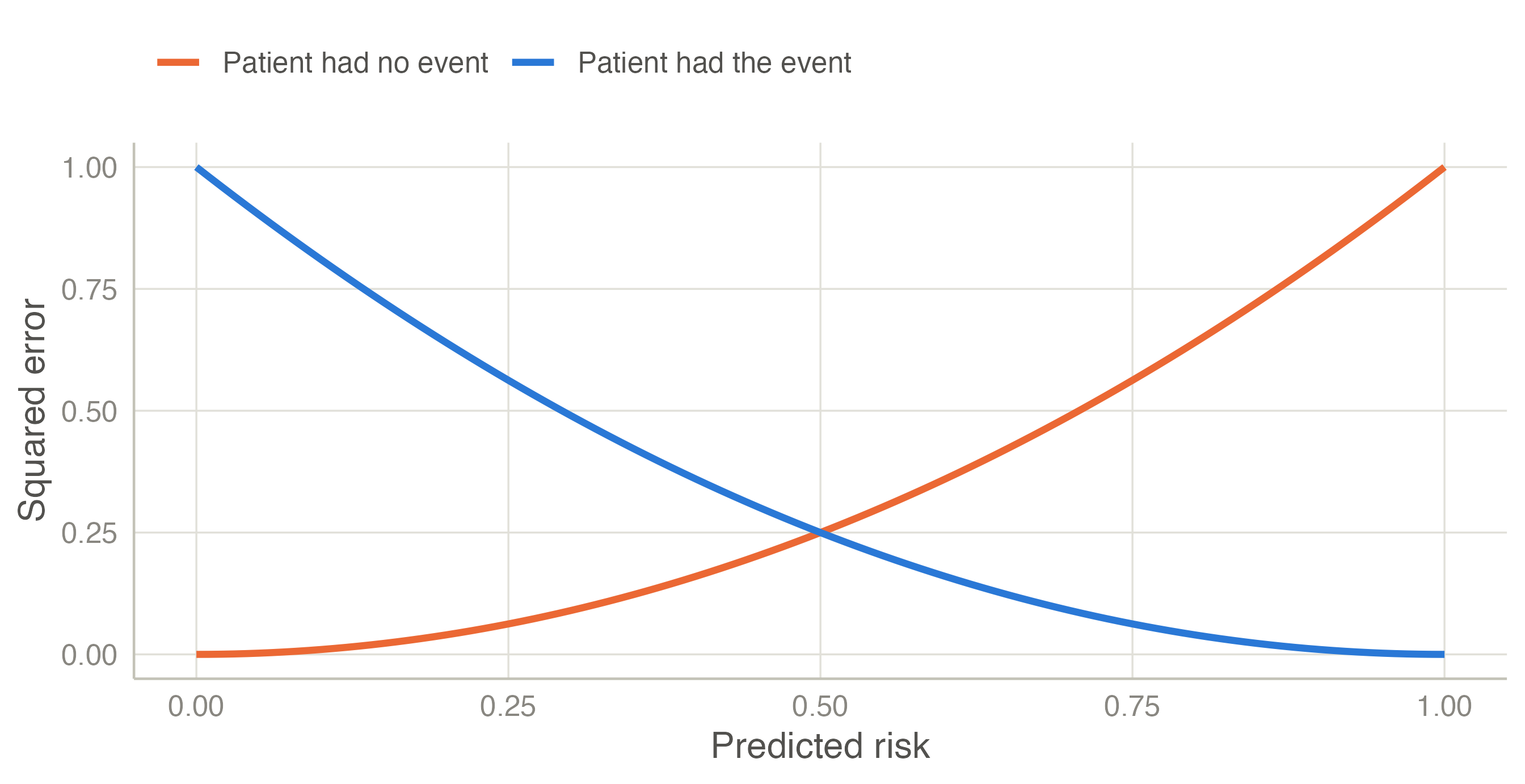
The value of a Brier score depends on how common the outcome is, so it needs a reference: a “model” without predictors that gives everyone the average risk (15.4% here) has a Brier score of 15.4% × (1 − 15.4%) = 0.1304. The heart model scores 0.1220. The scaled Brier score is the improvement over that reference: 1 − 0.1220 / 0.1304 = 0.064. The model removes 6.4% of the prediction error of knowing only the average risk — small, as for most models of a long-term outcome built on a few variables, where much of what will happen to an individual is unpredictable. A negative scaled Brier in new patients means the model is worse than the average risk. For Cox models clinpred weights the Brier score for censoring at the horizon (the scaled version is the index of prediction accuracy (Graf et al. 1999; Kattan and Gerds 2018)).
Nagelkerke’s and Cox–Snell’s R² are likelihood-based alternatives; the Cox–Snell R² is the input of the sample size criteria. For a continuous outcome, R² is computed around the mean of the data where it is measured, so it can be negative in validation data; RMSE and MAE are in the units of the outcome.
A good AUC and good calibration do not tell whether using the model helps. Models are used to decide: treat or not, test further or reassure. The question is whether deciding with the model leads to better decisions than the simple alternatives — treat everyone or treat no one.
Suppose a statin is offered to patients whose 10-year risk is above 20%. Choosing 20% means: for a patient at exactly 20% risk, treating and not treating are equally good. At that risk, out of 5 such patients 1 will have the event and 4 will not; being indifferent means that the benefit of treating the 1 is judged worth the harm (side effects, cost) of treating the 4. So the threshold fixes an exchange rate between false positives and true positives:
| Threshold | Odds t / (1 − t) | One true positive is worth |
|---|---|---|
| 5% | 1 : 19 | treating 19 patients unnecessarily |
| 10% | 1 : 9 | treating 9 unnecessarily |
| 20% | 1 : 4 | treating 4 unnecessarily |
| 33% | 1 : 2 | treating 2 unnecessarily |
| 50% | 1 : 1 | treating 1 unnecessarily |
A low threshold suits a cheap, safe intervention; a high one, a risky or expensive one.
Net benefit counts the true positives and subtracts the false positives, converted with the exchange rate, per patient (Vickers and Elkin 2006):
\[\text{Net benefit} = \frac{\text{TP}}{N} - \frac{\text{FP}}{N}\times\frac{t}{1-t}.\]
With the heart model at t = 20% (exchange rate 1 : 4), 577 of the 2360 patients are above the threshold: 164 of them had the event (true positives) and 413 did not (false positives). Net benefit = 164/2360 − 413/2360 × 0.25 = 0.0257: as if 2.6 patients per 100 were correctly treated with no one treated unnecessarily.
The alternatives: treat no one has net benefit 0 (no true, no false positives); treat everyone gets all 364 events but also all 1996 non-events: 364/2360 − 1996/2360 × 0.25 = -0.0572, negative — at this threshold, treating everyone does more harm than good. The model beats both, so at 20% deciding with the model is the best of the three strategies.
Different clinicians and patients choose different thresholds, so the calculation is repeated for every threshold:
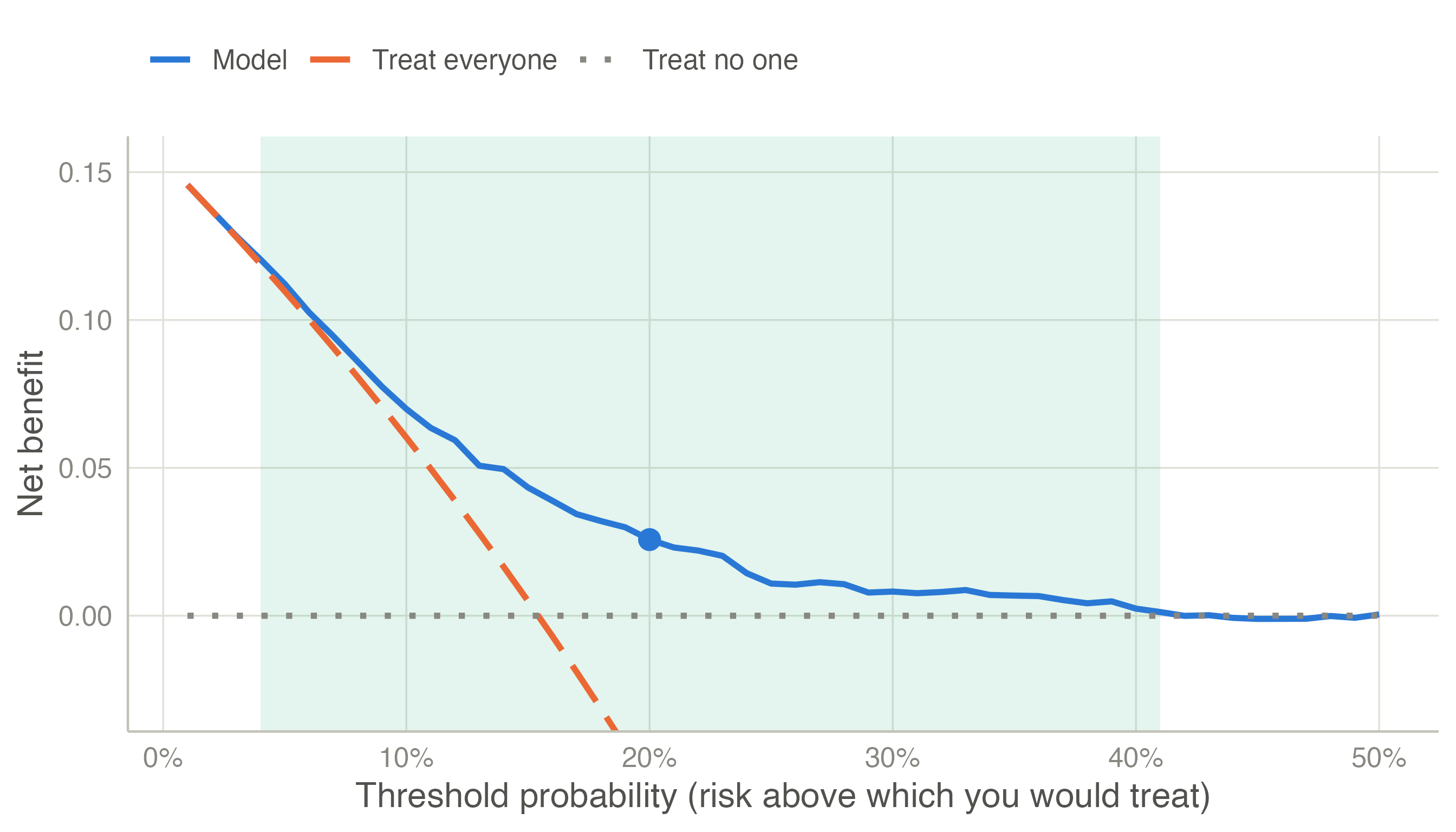
How to read it: at each threshold on the horizontal axis, the highest line is the best strategy. At very low thresholds (an intervention so safe that you would give it to almost anyone) treat everyone is as good as the model. From about 4% to 41% the model is best: in that range its predictions lead to better decisions. Where the model’s curve falls to the treat no one line, it identifies too few patients above the threshold to matter.
clinpred adds a table at chosen thresholds with the interventions avoided per 100 patients: how many fewer unnecessary treatments than treat everyone, for the same number of true positives — another way of saying the same thing. For Cox models, the risk of the event among the patients above each threshold is estimated by Kaplan–Meier at the horizon, so censoring is accounted for.
TRIPOD+AI (Collins et al. 2024) asks for discrimination and calibration (with a calibration plot) in the development data corrected for optimism, and in every validation; clinical utility when the model is meant to guide decisions. The reporting page maps each item to clinpred’s output.