Why matched data need a conditional analysis
Matching makes cases and controls alike on the matching factors, which removes their confounding by design, and the design has to be carried into the analysis. The model behind a matched study gives each matched set \(i\) its own baseline odds of being a case:
\[ \operatorname{logit} P(Y_{ij} = 1) = \alpha_i + \boldsymbol{x}_{ij}^\top \boldsymbol\beta, \]
where \(j\) indexes the subjects of set \(i\) and \(\boldsymbol\beta\) holds the log odds ratios of interest. The \(\alpha_i\) absorb everything shared within the set: the matching factors and whatever else they stand for.
Two analyses look natural and are both wrong:
The way out is to condition on what each set contributes to the design: the number of cases it contains. For a set with one case (subject 1) and \(M\) controls, the probability that the case is the subject it is, given that exactly one of the \(M+1\) is a case, is
\[ L_i(\boldsymbol\beta) = \frac{\exp(\boldsymbol{x}_{i1}^\top \boldsymbol\beta)} {\sum_{j=1}^{M+1} \exp(\boldsymbol{x}_{ij}^\top \boldsymbol\beta)}. \]
The \(\alpha_i\) cancel. The conditional likelihood is the product of the \(L_i\) over the sets, and maximising it gives consistent estimates of \(\boldsymbol\beta\) however many sets there are (Breslow et al. 1978). With \(k\) cases in a set the denominator runs over all \(\binom{M+k}{k}\) ways of choosing \(k\) subjects from the set.
\(L_i\) has the form of the partial likelihood of a Cox model at a single event time: the case is “the one who failed” and its set is the risk set. So a conditional logistic regression is a Cox model stratified by matched set, in which every subject has the same follow-up time and the cases are the events. With several cases per set they are events tied at that time, and the exact treatment of ties is exactly the conditional likelihood above (Gail et al. 1981). That is what R’s survival::clogit does, and what this module does:
coxph(Surv(rep(1, n), case) ~ x1 + x2 + strata(set), method = "exact")The Likelihood option of the Matching box chooses how ties are handled:
| Option | What it is | When |
|---|---|---|
| Exact conditional (default) | the conditional likelihood itself | always correct |
| Efron approximation | Efron’s approximation to it | sets with many cases, where the exact sum gets slow |
| Breslow approximation | Breslow’s approximation to it | the same, cruder |
With one case per set (1:1 or 1:M matching) there are no ties, and the three give identical results. They differ only when a set holds several cases.
For example, with 60 simulated sets of 2 cases and 4 controls, the log odds ratio of a continuous exposure is (exact), (Efron) and (Breslow): both approximations are attenuated towards zero, Breslow’s more. With a third of each set being cases this is a large share of ties, so keep the exact likelihood unless it is too slow.
Everything shared within a set is absorbed by the \(\alpha_i\), and so:
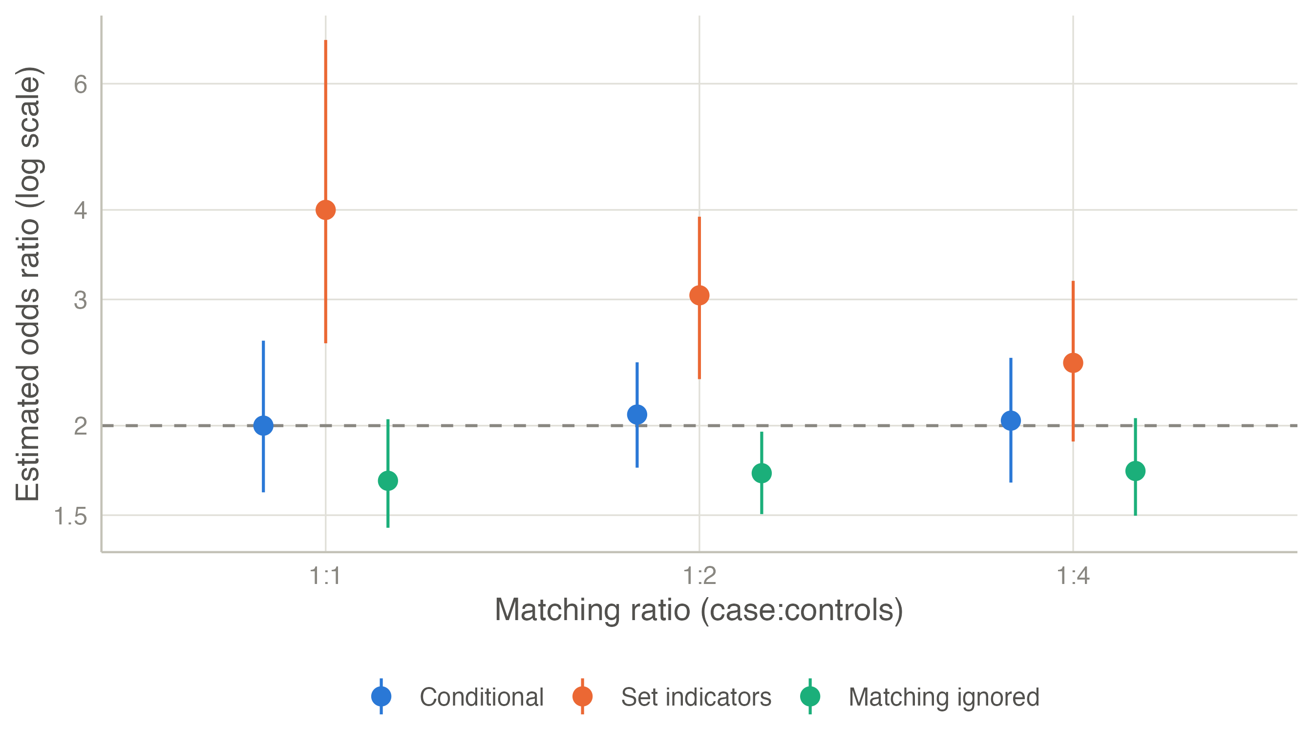
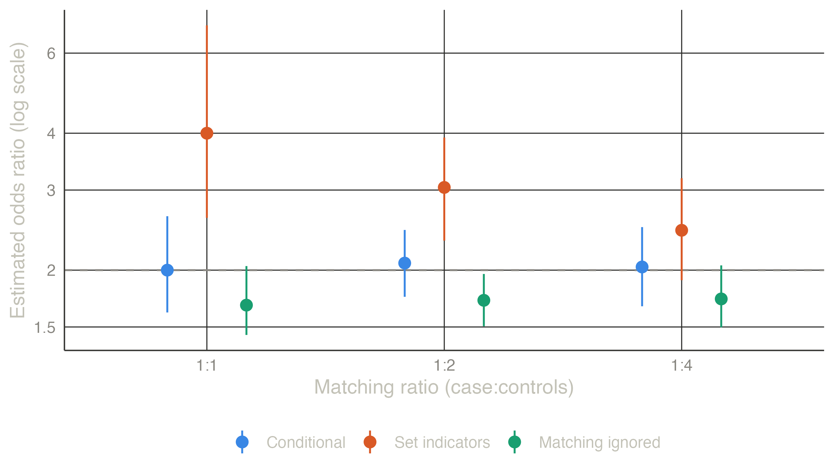
The figure shows 200 simulated studies for each matching ratio, with 100 matched sets each. The true odds ratio of a binary exposure is 2 (dashed line), and the matching factor is strongly related to the exposure. Points are median estimates; bars span the quartiles.
The conditional estimate is centred on the truth at every ratio. With set indicators the odds ratio is about squared for pairs, and the bias shrinks as more controls are matched to each case. Ignoring the matching biases the estimate towards 1 at every ratio.